
Hooke’s law: the force is proportional to the extension

Bourdon tubes are based on Hooke’s law. The force created by gas pressure inside the coiled metal tube above unwinds it by an amount proportional to the pressure.
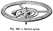
The balance wheel at the core of many mechanical clocks and watches depends on Hooke’s law. Since the torque generated by the coiled spring is proportional to the angle turned by the wheel, its oscillations have a nearly constant period.
In physics, Hooke’s law is an empirical law which states that the force (F) needed to extend or compress a spring by some distance (x) scales linearly with respect to that distance—that is, Fs = kx, where k is a constant factor characteristic of the spring (i.e., its stiffness), and x is small compared to the total possible deformation of the spring. The law is named after 17th-century British physicist Robert Hooke. He first stated the law in 1676 as a Latin anagram.[1][2] He published the solution of his anagram in 1678[3] as: ut tensio, sic vis («as the extension, so the force» or «the extension is proportional to the force»). Hooke states in the 1678 work that he was aware of the law since 1660.
Hooke’s equation holds (to some extent) in many other situations where an elastic body is deformed, such as wind blowing on a tall building, and a musician plucking a string of a guitar. An elastic body or material for which this equation can be assumed is said to be linear-elastic or Hookean.
Hooke’s law is only a first-order linear approximation to the real response of springs and other elastic bodies to applied forces. It must eventually fail once the forces exceed some limit, since no material can be compressed beyond a certain minimum size, or stretched beyond a maximum size, without some permanent deformation or change of state. Many materials will noticeably deviate from Hooke’s law well before those elastic limits are reached.
On the other hand, Hooke’s law is an accurate approximation for most solid bodies, as long as the forces and deformations are small enough. For this reason, Hooke’s law is extensively used in all branches of science and engineering, and is the foundation of many disciplines such as seismology, molecular mechanics and acoustics. It is also the fundamental principle behind the spring scale, the manometer, the galvanometer, and the balance wheel of the mechanical clock.
The modern theory of elasticity generalizes Hooke’s law to say that the strain (deformation) of an elastic object or material is proportional to the stress applied to it. However, since general stresses and strains may have multiple independent components, the «proportionality factor» may no longer be just a single real number, but rather a linear map (a tensor) that can be represented by a matrix of real numbers.
In this general form, Hooke’s law makes it possible to deduce the relation between strain and stress for complex objects in terms of intrinsic properties of the materials they are made of. For example, one can deduce that a homogeneous rod with uniform cross section will behave like a simple spring when stretched, with a stiffness k directly proportional to its cross-section area and inversely proportional to its length.
Formal definition
For linear springs
Consider a simple helical spring that has one end attached to some fixed object, while the free end is being pulled by a force whose magnitude is Fs. Suppose that the spring has reached a state of equilibrium, where its length is not changing anymore. Let x be the amount by which the free end of the spring was displaced from its «relaxed» position (when it is not being stretched). Hooke’s law states that

or, equivalently,

where k is a positive real number, characteristic of the spring. Moreover, the same formula holds when the spring is compressed, with Fs and x both negative in that case. According to this formula, the graph of the applied force Fs as a function of the displacement x will be a straight line passing through the origin, whose slope is k.
Hooke’s law for a spring is sometimes, but rarely, stated under the convention that Fs is the restoring force exerted by the spring on whatever is pulling its free end. In that case, the equation becomes

since the direction of the restoring force is opposite to that of the displacement.
General «scalar» springs
Hooke’s spring law usually applies to any elastic object, of arbitrary complexity, as long as both the deformation and the stress can be expressed by a single number that can be both positive and negative.
For example, when a block of rubber attached to two parallel plates is deformed by shearing, rather than stretching or compression, the shearing force Fs and the sideways displacement of the plates x obey Hooke’s law (for small enough deformations).
Hooke’s law also applies when a straight steel bar or concrete beam (like the one used in buildings), supported at both ends, is bent by a weight F placed at some intermediate point. The displacement x in this case is the deviation of the beam, measured in the transversal direction, relative to its unloaded shape.
The law also applies when a stretched steel wire is twisted by pulling on a lever attached to one end. In this case the stress Fs can be taken as the force applied to the lever, and x as the distance traveled by it along its circular path. Or, equivalently, one can let Fs be the torque applied by the lever to the end of the wire, and x be the angle by which that end turns. In either case Fs is proportional to x (although the constant k is different in each case.)
Vector formulation
In the case of a helical spring that is stretched or compressed along its axis, the applied (or restoring) force and the resulting elongation or compression have the same direction (which is the direction of said axis). Therefore, if Fs and x are defined as vectors, Hooke’s equation still holds and says that the force vector is the elongation vector multiplied by a fixed scalar.
General tensor form
Some elastic bodies will deform in one direction when subjected to a force with a different direction. One example is a horizontal wood beam with non-square rectangular cross section that is bent by a transverse load that is neither vertical nor horizontal. In such cases, the magnitude of the displacement x will be proportional to the magnitude of the force Fs, as long as the direction of the latter remains the same (and its value is not too large); so the scalar version of Hooke’s law Fs = −kx will hold. However, the force and displacement vectors will not be scalar multiples of each other, since they have different directions. Moreover, the ratio k between their magnitudes will depend on the direction of the vector Fs.
Yet, in such cases there is often a fixed linear relation between the force and deformation vectors, as long as they are small enough. Namely, there is a function κ from vectors to vectors, such that F = κ(X), and κ(αX1 + βX2) = ακ(X1) + βκ(X2) for any real numbers α, β and any displacement vectors X1, X2. Such a function is called a (second-order) tensor.
With respect to an arbitrary Cartesian coordinate system, the force and displacement vectors can be represented by 3 × 1 matrices of real numbers. Then the tensor κ connecting them can be represented by a 3 × 3 matrix κ of real coefficients, that, when multiplied by the displacement vector, gives the force vector:

That is,

for i = 1, 2, 3. Therefore, Hooke’s law F = κX can be said to hold also when X and F are vectors with variable directions, except that the stiffness of the object is a tensor κ, rather than a single real number k.
Hooke’s law for continuous media

(a) Schematic of a polymer nanospring. The coil radius, R, pitch, P, length of the spring, L, and the number of turns, N, are 2.5 μm, 2.0 μm, 13 μm, and 4, respectively. Electron micrographs of the nanospring, before loading (b-e), stretched (f), compressed (g), bent (h), and recovered (i). All scale bars are 2 μm. The spring followed a linear response against applied force, demonstrating the validity of Hooke’s law at the nanoscale.[4]
The stresses and strains of the material inside a continuous elastic material (such as a block of rubber, the wall of a boiler, or a steel bar) are connected by a linear relationship that is mathematically similar to Hooke’s spring law, and is often referred to by that name.
However, the strain state in a solid medium around some point cannot be described by a single vector. The same parcel of material, no matter how small, can be compressed, stretched, and sheared at the same time, along different directions. Likewise, the stresses in that parcel can be at once pushing, pulling, and shearing.
In order to capture this complexity, the relevant state of the medium around a point must be represented by two-second-order tensors, the strain tensor ε (in lieu of the displacement X) and the stress tensor σ (replacing the restoring force F). The analogue of Hooke’s spring law for continuous media is then

where c is a fourth-order tensor (that is, a linear map between second-order tensors) usually called the stiffness tensor or elasticity tensor. One may also write it as

where the tensor s, called the compliance tensor, represents the inverse of said linear map.
In a Cartesian coordinate system, the stress and strain tensors can be represented by 3 × 3 matrices

Being a linear mapping between the nine numbers σij and the nine numbers εkl, the stiffness tensor c is represented by a matrix of 3 × 3 × 3 × 3 = 81 real numbers cijkl. Hooke’s law then says that

where i,j = 1,2,3.
All three tensors generally vary from point to point inside the medium, and may vary with time as well. The strain tensor ε merely specifies the displacement of the medium particles in the neighborhood of the point, while the stress tensor σ specifies the forces that neighboring parcels of the medium are exerting on each other. Therefore, they are independent of the composition and physical state of the material. The stiffness tensor c, on the other hand, is a property of the material, and often depends on physical state variables such as temperature, pressure, and microstructure.
Due to the inherent symmetries of σ, ε, and c, only 21 elastic coefficients of the latter are independent.[5] This number can be further reduced by the symmetry of the material: 9 for an orthorhombic crystal, 5 for an hexagonal structure, and 3 for a cubic symmetry.[6] For isotropic media (which have the same physical properties in any direction), c can be reduced to only two independent numbers, the bulk modulus K and the shear modulus G, that quantify the material’s resistance to changes in volume and to shearing deformations, respectively.
Analogous laws
Since Hooke’s law is a simple proportionality between two quantities, its formulas and consequences are mathematically similar to those of many other physical laws, such as those describing the motion of fluids, or the polarization of a dielectric by an electric field.
In particular, the tensor equation σ = cε relating elastic stresses to strains is entirely similar to the equation τ = με̇ relating the viscous stress tensor τ and the strain rate tensor ε̇ in flows of viscous fluids; although the former pertains to static stresses (related to amount of deformation) while the latter pertains to dynamical stresses (related to the rate of deformation).
Units of measurement
In SI units, displacements are measured in meters (m), and forces in newtons (N or kg·m/s2). Therefore, the spring constant k, and each element of the tensor κ, is measured in newtons per meter (N/m), or kilograms per second squared (kg/s2).
For continuous media, each element of the stress tensor σ is a force divided by an area; it is therefore measured in units of pressure, namely pascals (Pa, or N/m2, or kg/(m·s2). The elements of the strain tensor ε are dimensionless (displacements divided by distances). Therefore, the entries of cijkl are also expressed in units of pressure.
General application to elastic materials

Objects that quickly regain their original shape after being deformed by a force, with the molecules or atoms of their material returning to the initial state of stable equilibrium, often obey Hooke’s law.
Hooke’s law only holds for some materials under certain loading conditions. Steel exhibits linear-elastic behavior in most engineering applications; Hooke’s law is valid for it throughout its elastic range (i.e., for stresses below the yield strength). For some other materials, such as aluminium, Hooke’s law is only valid for a portion of the elastic range. For these materials a proportional limit stress is defined, below which the errors associated with the linear approximation are negligible.
Rubber is generally regarded as a «non-Hookean» material because its elasticity is stress dependent and sensitive to temperature and loading rate.
Generalizations of Hooke’s law for the case of large deformations is provided by models of neo-Hookean solids and Mooney–Rivlin solids.
Derived formulae
Tensional stress of a uniform bar
A rod of any elastic material may be viewed as a linear spring. The rod has length L and cross-sectional area A. Its tensile stress σ is linearly proportional to its fractional extension or strain ε by the modulus of elasticity E:

The modulus of elasticity may often be considered constant. In turn,

(that is, the fractional change in length), and since

it follows that:

The change in length may be expressed as

Spring energy
The potential energy Uel(x) stored in a spring is given by

which comes from adding up the energy it takes to incrementally compress the spring. That is, the integral of force over displacement. Since the external force has the same general direction as the displacement, the potential energy of a spring is always non-negative.
This potential Uel can be visualized as a parabola on the Ux-plane such that Uel(x) = 1/2kx2. As the spring is stretched in the positive x-direction, the potential energy increases parabolically (the same thing happens as the spring is compressed). Since the change in potential energy changes at a constant rate:

Note that the change in the change in U is constant even when the displacement and acceleration are zero.
Relaxed force constants (generalized compliance constants)
Relaxed force constants (the inverse of generalized compliance constants) are uniquely defined for molecular systems, in contradistinction to the usual «rigid» force constants, and thus their use allows meaningful correlations to be made between force fields calculated for reactants, transition states, and products of a chemical reaction. Just as the potential energy can be written as a quadratic form in the internal coordinates, so it can also be written in terms of generalized forces. The resulting coefficients are termed compliance constants. A direct method exists for calculating the compliance constant for any internal coordinate of a molecule, without the need to do the normal mode analysis.[7] The suitability of relaxed force constants (inverse compliance constants) as covalent bond strength descriptors was demonstrated as early as 1980. Recently, the suitability as non-covalent bond strength descriptors was demonstrated too.[8]
Harmonic oscillator
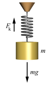
A mass suspended by a spring is the classical example of a harmonic oscillator
A mass m attached to the end of a spring is a classic example of a harmonic oscillator. By pulling slightly on the mass and then releasing it, the system will be set in sinusoidal oscillating motion about the equilibrium position. To the extent that the spring obeys Hooke’s law, and that one can neglect friction and the mass of the spring, the amplitude of the oscillation will remain constant; and its frequency f will be independent of its amplitude, determined only by the mass and the stiffness of the spring:

This phenomenon made possible the construction of accurate mechanical clocks and watches that could be carried on ships and people’s pockets.
Rotation in gravity-free space
If the mass m were attached to a spring with force constant k and rotating in free space, the spring tension (Ft) would supply the required centripetal force (Fc):

Since Ft = Fc and x = r, then:

Given that ω = 2πf, this leads to the same frequency equation as above:
Linear elasticity theory for continuous media
- Note: the Einstein summation convention of summing on repeated indices is used below.
Isotropic materials
For an analogous development for viscous fluids, see Viscosity.
Isotropic materials are characterized by properties which are independent of direction in space. Physical equations involving isotropic materials must therefore be independent of the coordinate system chosen to represent them. The strain tensor is a symmetric tensor. Since the trace of any tensor is independent of any coordinate system, the most complete coordinate-free decomposition of a symmetric tensor is to represent it as the sum of a constant tensor and a traceless symmetric tensor.[9] Thus in index notation:

where δij is the Kronecker delta. In direct tensor notation:

where I is the second-order identity tensor.
The first term on the right is the constant tensor, also known as the volumetric strain tensor, and the second term is the traceless symmetric tensor, also known as the deviatoric strain tensor or shear tensor.
The most general form of Hooke’s law for isotropic materials may now be written as a linear combination of these two tensors:

where K is the bulk modulus and G is the shear modulus.
Using the relationships between the elastic moduli, these equations may also be expressed in various other ways. A common form of Hooke’s law for isotropic materials, expressed in direct tensor notation, is
[10]

where λ = K − 2/3G = c1111 − 2c1212 and μ = G = c1212 are the Lamé constants, I is the second-rank identity tensor, and I is the symmetric part of the fourth-rank identity tensor. In index notation:

The inverse relationship is[11]

Therefore, the compliance tensor in the relation ε = s : σ is

In terms of Young’s modulus and Poisson’s ratio, Hooke’s law for isotropic materials can then be expressed as

This is the form in which the strain is expressed in terms of the stress tensor in engineering. The expression in expanded form is

where E is Young’s modulus and ν is Poisson’s ratio. (See 3-D elasticity).
Derivation of Hooke’s law in three dimensions
The three-dimensional form of Hooke’s law can be derived using Poisson’s ratio and the one-dimensional form of Hooke’s law as follows.
Consider the strain and stress relation as a superposition of two effects: stretching in direction of the load (1) and shrinking (caused by the load) in perpendicular directions (2 and 3),

where ν is Poisson’s ratio and E is Young’s modulus.
We get similar equations to the loads in directions 2 and 3,

and

Summing the three cases together (εi = εi′ + εi″ + εi‴) we get

or by adding and subtracting one νσ

and further we get by solving σ1

Calculating the sum

and substituting it to the equation solved for σ1 gives

where μ and λ are the Lamé parameters.
Similar treatment of directions 2 and 3 gives the Hooke’s law in three dimensions.
In matrix form, Hooke’s law for isotropic materials can be written as

where γij = 2εij is the engineering shear strain. The inverse relation may be written as

which can be simplified thanks to the Lamé constants:

In vector notation this becomes

where I is the identity tensor.
Plane stress
Under plane stress conditions, σ31 = σ13 = σ32 = σ23 = σ33 = 0. In that case Hooke’s law takes the form

In vector notation this becomes

The inverse relation is usually written in the reduced form

Plane strain
Under plane strain conditions, ε31 = ε13 = ε32 = ε23 = ε33 = 0. In this case Hooke’s law takes the form

Anisotropic materials
The symmetry of the Cauchy stress tensor (σij = σji) and the generalized Hooke’s laws (σij = cijklεkl) implies that cijkl = cjikl. Similarly, the symmetry of the infinitesimal strain tensor implies that cijkl = cijlk. These symmetries are called the minor symmetries of the stiffness tensor c. This reduces the number of elastic constants from 81 to 36.
If in addition, since the displacement gradient and the Cauchy stress are work conjugate, the stress–strain relation can be derived from a strain energy density functional (U), then

The arbitrariness of the order of differentiation implies that cijkl = cklij. These are called the major symmetries of the stiffness tensor. This reduces the number of elastic constants from 36 to 21. The major and minor symmetries indicate that the stiffness tensor has only 21 independent components.
Matrix representation (stiffness tensor)
It is often useful to express the anisotropic form of Hooke’s law in matrix notation, also called Voigt notation. To do this we take advantage of the symmetry of the stress and strain tensors and express them as six-dimensional vectors in an orthonormal coordinate system (e1,e2,e3) as
![{displaystyle [{boldsymbol {sigma }}],=,{begin{bmatrix}sigma _{11}\sigma _{22}\sigma _{33}\sigma _{23}\sigma _{13}\sigma _{12}end{bmatrix}},equiv ,{begin{bmatrix}sigma _{1}\sigma _{2}\sigma _{3}\sigma _{4}\sigma _{5}\sigma _{6}end{bmatrix}},;qquad [{boldsymbol {varepsilon }}],=,{begin{bmatrix}varepsilon _{11}\varepsilon _{22}\varepsilon _{33}\2varepsilon _{23}\2varepsilon _{13}\2varepsilon _{12}end{bmatrix}},equiv ,{begin{bmatrix}varepsilon _{1}\varepsilon _{2}\varepsilon _{3}\varepsilon _{4}\varepsilon _{5}\varepsilon _{6}end{bmatrix}}}](https://wikimedia.org/api/rest_v1/media/math/render/svg/99d84c34fc9efc62922b42a33f888656c62d794b)
Then the stiffness tensor (c) can be expressed as
![{displaystyle [{mathsf {c}}],=,{begin{bmatrix}c_{1111}&c_{1122}&c_{1133}&c_{1123}&c_{1131}&c_{1112}\c_{2211}&c_{2222}&c_{2233}&c_{2223}&c_{2231}&c_{2212}\c_{3311}&c_{3322}&c_{3333}&c_{3323}&c_{3331}&c_{3312}\c_{2311}&c_{2322}&c_{2333}&c_{2323}&c_{2331}&c_{2312}\c_{3111}&c_{3122}&c_{3133}&c_{3123}&c_{3131}&c_{3112}\c_{1211}&c_{1222}&c_{1233}&c_{1223}&c_{1231}&c_{1212}end{bmatrix}},equiv ,{begin{bmatrix}C_{11}&C_{12}&C_{13}&C_{14}&C_{15}&C_{16}\C_{12}&C_{22}&C_{23}&C_{24}&C_{25}&C_{26}\C_{13}&C_{23}&C_{33}&C_{34}&C_{35}&C_{36}\C_{14}&C_{24}&C_{34}&C_{44}&C_{45}&C_{46}\C_{15}&C_{25}&C_{35}&C_{45}&C_{55}&C_{56}\C_{16}&C_{26}&C_{36}&C_{46}&C_{56}&C_{66}end{bmatrix}}}](https://wikimedia.org/api/rest_v1/media/math/render/svg/85c8bf05adff9dcaec56f4863dd039fae5986a79)
and Hooke’s law is written as
![{displaystyle [{boldsymbol {sigma }}]=[{mathsf {C}}][{boldsymbol {varepsilon }}]qquad {text{or}}qquad sigma _{i}=C_{ij}varepsilon _{j},.}](https://wikimedia.org/api/rest_v1/media/math/render/svg/2f0315b5cfc25f83e499fadf8ce4921e11340f8e)
Similarly the compliance tensor (s) can be written as
![{displaystyle [{mathsf {s}}],=,{begin{bmatrix}s_{1111}&s_{1122}&s_{1133}&2s_{1123}&2s_{1131}&2s_{1112}\s_{2211}&s_{2222}&s_{2233}&2s_{2223}&2s_{2231}&2s_{2212}\s_{3311}&s_{3322}&s_{3333}&2s_{3323}&2s_{3331}&2s_{3312}\2s_{2311}&2s_{2322}&2s_{2333}&4s_{2323}&4s_{2331}&4s_{2312}\2s_{3111}&2s_{3122}&2s_{3133}&4s_{3123}&4s_{3131}&4s_{3112}\2s_{1211}&2s_{1222}&2s_{1233}&4s_{1223}&4s_{1231}&4s_{1212}end{bmatrix}},equiv ,{begin{bmatrix}S_{11}&S_{12}&S_{13}&S_{14}&S_{15}&S_{16}\S_{12}&S_{22}&S_{23}&S_{24}&S_{25}&S_{26}\S_{13}&S_{23}&S_{33}&S_{34}&S_{35}&S_{36}\S_{14}&S_{24}&S_{34}&S_{44}&S_{45}&S_{46}\S_{15}&S_{25}&S_{35}&S_{45}&S_{55}&S_{56}\S_{16}&S_{26}&S_{36}&S_{46}&S_{56}&S_{66}end{bmatrix}}}](https://wikimedia.org/api/rest_v1/media/math/render/svg/34760b2d8ef86f720051aebe5a45a65b312bcab6)
Change of coordinate system
If a linear elastic material is rotated from a reference configuration to another, then the material is symmetric with respect to the rotation if the components of the stiffness tensor in the rotated configuration are related to the components in the reference configuration by the relation[12]

where lab are the components of an orthogonal rotation matrix [L]. The same relation also holds for inversions.
In matrix notation, if the transformed basis (rotated or inverted) is related to the reference basis by
![{displaystyle [mathbf {e} _{i}']=[L][mathbf {e} _{i}]}](https://wikimedia.org/api/rest_v1/media/math/render/svg/213d0bb55cc1da894c855871790e09d78635c17b)
then

In addition, if the material is symmetric with respect to the transformation [L] then

Orthotropic materials
Orthotropic materials have three orthogonal planes of symmetry. If the basis vectors (e1,e2,e3) are normals to the planes of symmetry then the coordinate transformation relations imply that

The inverse of this relation is commonly written as[13][page needed]

where
- Ei is the Young’s modulus along axis i
- Gij is the shear modulus in direction j on the plane whose normal is in direction i
- νij is the Poisson’s ratio that corresponds to a contraction in direction j when an extension is applied in direction i.
Under plane stress conditions, σzz = σzx = σyz = 0, Hooke’s law for an orthotropic material takes the form

The inverse relation is

The transposed form of the above stiffness matrix is also often used.
Transversely isotropic materials
A transversely isotropic material is symmetric with respect to a rotation about an axis of symmetry. For such a material, if e3 is the axis of symmetry, Hooke’s law can be expressed as

More frequently, the x ≡ e1 axis is taken to be the axis of symmetry and the inverse Hooke’s law is written as
[14]

Universal elastic anisotropy index
To grasp the degree of anisotropy of any class, a universal elastic anisotropy index (AU)[15] was formulated. It replaces the Zener ratio, which is suited for cubic crystals.
Thermodynamic basis
Linear deformations of elastic materials can be approximated as adiabatic. Under these conditions and for quasistatic processes the first law of thermodynamics for a deformed body can be expressed as

where δU is the increase in internal energy and δW is the work done by external forces. The work can be split into two terms

where δWs is the work done by surface forces while δWb is the work done by body forces. If δu is a variation of the displacement field u in the body, then the two external work terms can be expressed as

where t is the surface traction vector, b is the body force vector, Ω represents the body and ∂Ω represents its surface. Using the relation between the Cauchy stress and the surface traction, t = n · σ (where n is the unit outward normal to ∂Ω), we have

Converting the surface integral into a volume integral via the divergence theorem gives

Using the symmetry of the Cauchy stress and the identity

we have the following

From the definition of strain and from the equations of equilibrium we have

Hence we can write

and therefore the variation in the internal energy density is given by

An elastic material is defined as one in which the total internal energy is equal to the potential energy of the internal forces (also called the elastic strain energy). Therefore, the internal energy density is a function of the strains, U0 = U0(ε) and the variation of the internal energy can be expressed as

Since the variation of strain is arbitrary, the stress–strain relation of an elastic material is given by

For a linear elastic material, the quantity ∂U0/∂ε is a linear function of ε, and can therefore be expressed as

where c is a fourth-rank tensor of material constants, also called the stiffness tensor. We can see why c must be a fourth-rank tensor by noting that, for a linear elastic material,

In index notation

The right-hand side constant requires four indices and is a fourth-rank quantity. We can also see that this quantity must be a tensor because it is a linear transformation that takes the strain tensor to the stress tensor. We can also show that the constant obeys the tensor transformation rules for fourth-rank tensors.
See also
- Acoustoelastic effect
- Elastic potential energy
- Laws of science
- List of scientific laws named after people
- Quadratic form
- Series and parallel springs
- Spring system
- Simple harmonic motion of a mass on a spring
- Sine wave
- Solid mechanics
- Spring pendulum
Notes
- ^ The anagram was given in alphabetical order, ceiiinosssttuu, representing Ut tensio, sic vis – «As the extension, so the force»: Petroski, Henry (1996). Invention by Design: How Engineers Get from Thought to Thing. Cambridge, MA: Harvard University Press. p. 11. ISBN 978-0674463684.
- ^ See http://civil.lindahall.org/design.shtml, where one can find also an anagram for catenary.
- ^ Robert Hooke, De Potentia Restitutiva, or of Spring. Explaining the Power of Springing Bodies, London, 1678.
- ^ Ushiba, Shota; Masui, Kyoko; Taguchi, Natsuo; Hamano, Tomoki; Kawata, Satoshi; Shoji, Satoru (2015). «Size dependent nanomechanics of coil spring shaped polymer nanowires». Scientific Reports. 5: 17152. Bibcode:2015NatSR…517152U. doi:10.1038/srep17152. PMC 4661696. PMID 26612544.
- ^ Belen’kii; Salaev (1988). «Deformation effects in layer crystals». Uspekhi Fizicheskikh Nauk. 155 (5): 89. doi:10.3367/UFNr.0155.198805c.0089.
- ^ Mouhat, Félix; Coudert, François-Xavier (5 December 2014). «Necessary and sufficient elastic stability conditions in various crystal systems». Physical Review B. 90 (22): 224104. arXiv:1410.0065. Bibcode:2014PhRvB..90v4104M. doi:10.1103/PhysRevB.90.224104. ISSN 1098-0121. S2CID 54058316.
- ^ Vijay Madhav, M.; Manogaran, S. (2009). «A relook at the compliance constants in redundant internal coordinates and some new insights». J. Chem. Phys. 131 (17): 174112–174116. Bibcode:2009JChPh.131q4112V. doi:10.1063/1.3259834. PMID 19895003.
- ^ Ponomareva, Alla; Yurenko, Yevgen; Zhurakivsky, Roman; Van Mourik, Tanja; Hovorun, Dmytro (2012). «Complete conformational space of the potential HIV-1 reverse transcriptase inhibitors d4U and d4C. A quantum chemical study». Phys. Chem. Chem. Phys. 14 (19): 6787–6795. Bibcode:2012PCCP…14.6787P. doi:10.1039/C2CP40290D. PMID 22461011.
- ^ Symon, Keith R. (1971). «Chapter 10». Mechanics. Reading, Massachusetts: Addison-Wesley. ISBN 9780201073928.
- ^ Simo, J. C.; Hughes, T. J. R. (1998). Computational Inelasticity. Springer. ISBN 9780387975207.
- ^ Milton, Graeme W. (2002). The Theory of Composites. Cambridge Monographs on Applied and Computational Mathematics. Cambridge University Press. ISBN 9780521781251.
- ^ Slaughter, William S. (2001). The Linearized Theory of Elasticity. Birkhäuser. ISBN 978-0817641177.
- ^ Boresi, A. P.; Schmidt, R. J.; Sidebottom, O. M. (1993). Advanced Mechanics of Materials (5th ed.). Wiley. ISBN 9780471600091.
- ^ Tan, S. C. (1994). Stress Concentrations in Laminated Composites. Lancaster, PA: Technomic Publishing Company. ISBN 9781566760775.
- ^ Ranganathan, S.I.; Ostoja-Starzewski, M. (2008). «Universal Elastic Anisotropy Index». Physical Review Letters. 101 (5): 055504–1–4. Bibcode:2008PhRvL.101e5504R. doi:10.1103/PhysRevLett.101.055504. PMID 18764407.
References
- Hooke’s law — The Feynman Lectures on Physics
- Hooke’s Law — Classical Mechanics — Physics — MIT OpenCourseWare
External links
- JavaScript Applet demonstrating Springs and Hooke’s law
- JavaScript Applet demonstrating Spring Force
| Conversion formulae | |||||||
|---|---|---|---|---|---|---|---|
| Homogeneous isotropic linear elastic materials have their elastic properties uniquely determined by any two moduli among these; thus, given any two, any other of the elastic moduli can be calculated according to these formulas, provided both for 3D materials (first part of the table) and for 2D materials (second part). | |||||||
| 3D formulae | 
|

|

|

|

|

|
Notes |

|

|

|

|

|
|||

|

|

|

|

|
|||

|

|

|

|

|
|||

|

|

|

|

|
|||

|

|

|

|

|
|||

|

|

|

|

|

|
||

|

|

|

|

|
|||

|

|

|

|

|
|||

|

|

|

|

|

There are two valid solutions. The minus sign leads to |
||

|

|

|

|

|
|||

|

|

|

|

|
Cannot be used when 
|
||

|

|

|

|

|
|||

|

|

|

|

|
|||

|

|

|

|

|
|||

|

|

|

|

|
|||
| 2D formulae | 
|

|

|

|

|

|
Notes |

|

|

|

|

|
|||

|

|

|

|

|
|||

|

|

|

|

|
|||

|

|

|

|

|
|||

|

|

|

|

|
|||

|

|

|

|

|
|||

|

|

|

|

|
|||

|

|

|

|

|
Cannot be used when 
|
||

|

|

|

|

|
|||

|

|

|

|

|


Физика, 10 класс
Урок 9. Закон Гука
Перечень вопросов, рассматриваемых на этом уроке
1.Закона Гука.
2.Модели видов деформаций.
3. Вычисление и измерение силы упругости, жёсткости и удлинение пружины.
Глоссарий по теме
Сила упругости – это сила, возникающая в теле в результате его деформации и стремящаяся вернуть тело в исходное положение.
Деформация – изменение формы или размеров тела, происходящее из-за неодинакового смещения различных частей одного и того же тела в результате воздействия другого тела. Виды деформаций: сжатие, растяжение, изгиб, сдвиг, кручение.
Закон Гука – сила упругости, возникающая при деформации тела (растяжение или сжатие пружины), пропорциональна удлинению тела (пружины), и направлена в сторону противоположную направлению перемещений частиц тела
Основная и дополнительная литература по теме:
Г.Я. Мякишев., Б.Б.Буховцев., Н.Н.Сотский. Физика.10 класс. Учебник для общеобразовательных организаций М.: Просвещение, 2017стр. 107-112
Рымкевич А.П. Сборник задач по физике. 10-11класс.- М.:Дрофа,2009. Стр 28-29
ЕГЭ 2017. Физика. 1000 задач с ответами и решениями. Демидова М.Ю., Грибов В.А., Гиголо А.И. М.: Экзамен, 2017.
Основное содержание урока
В окружающем нас мире мы наблюдаем, как различные силы заставляют тела двигаться, делать прыжки, перемещаться, взаимодействовать.
Однако можно также наблюдать как происходят разрушения, так называемые деформации, различных сооружений: мостов, домов, разнообразных машин.
Что необходимо знать инженеру конструктору, строителю, чтобы строить надёжные сооружения: дома, мосты, машины?
Почему деформации различны, какие виды деформации могут быть у конкретных тел? Почему одни тела после деформации могут восстановиться, а другие нет? От чего зависит и можно ли рассчитать величину этих деформаций?
Деформация — это изменение формы или размеров тела, в результате воздействия на него другого тела.
Почему деформации не одинаковы у различных тел, если мы их, к примеру, сжимаем? Давайте вспомним что мы знаем о строении вещества.
Все вещества состоят из частиц. Между этими частицами существуют силы взаимодействия- эти силы электромагнитной природы. Эти силы в зависимости от расстояний между частицами проявляются, то как силы притяжения, то как силы отталкивания.
Сила упругости – сила, возникающая при деформации любых тел, а также при сжатии жидкостей и газов. Она противодействует изменению формы тел.
Мы можем наблюдать несколько видов деформаций: сжатие, растяжение, изгиб, сдвиг, кручение.
При деформации растяжения межмолекулярные расстояния увеличиваются. Такую деформацию испытывают струны в музыкальных инструментах, различные нити, тросы, буксирные тросы.
При деформации сжатия межмолекулярные расстояния уменьшаются. Под такой деформацией находятся стены, фундаменты сооружений и зданий.
При деформации изгиба происходят неординарные изменения, одни межмолекулярные слои увеличиваются, а другие уменьшаются. Такие деформации испытывают перекрытия в зданиях и мостах.
При кручении – происходят повороты одних молекулярных слоёв относительно других. Эту деформацию испытывают: валы, витки цилиндрических пружин, столярный бур, свёрла по металлу, валы при бурении нефтяных скважин. Деформация среза тоже является разновидностью деформации сдвига.
Первое научное исследование упругого растяжения и сжатия вещества провёл английский учёный Роберт Гук.
Роберт Гук установил, что при малых деформациях растяжения или сжатия тела абсолютное удлинение тела прямо пропорционально деформирующей силе.

F упр = k ·Δℓ = k · Iℓ−ℓ0I закон Гука.
k− коэффициент пропорциональности, жёсткость тела.
ℓ0 — начальная длина.
ℓ — конечная длина после деформации.
Δℓ = I ℓ−ℓ₀ I- абсолютное удлинение пружины.
 — единица измерения жёсткости в системе СИ.
При больших деформациях изменение длины перестаёт быть прямо пропорциональным приложенной силе, а слишком большие деформации разрушают тело.
Для расчёта движения тел под действием силы упругости, нужно учитывать направление этой силы. Если принять за начало отсчёта крайнюю точку недеформированного тела, то абсолютное удлинение тела можно характеризовать конечной координатой деформированного тела. При растяжении и сжатии сила упругости направлена противоположно смещению его конца.
Закон Гука можно записать для проекции силы упругости на выбранную координатную ось в виде:
F упр x = − kx — закона Гука.
k – коэффициент пропорциональности, жёсткость тела.
x = Δℓ = ℓ−ℓ0 удлинение тела (пружины, резины, шнура, нити….)
Fупр x = − kx
Закон Гука:
Fупр = k·Δℓ = k · Iℓ−ℓ0I
Графиком зависимости модуля силы упругости от абсолютного удлинения тела является прямая, угол наклона которой к оси абсцисс зависит от коэффициента жёсткости k. Если прямая идёт круче к оси силы упругости, то коэффициент жёсткости этого тела больше, если же уклон прямой идёт ближе к оси абсолютного удлинения, следует понимать, что жёсткость тела меньше.

График, зависимости проекции силы упругости на ось ОХ, того же тела от значения х.

Необходимо помнить, что закон Гука хорошо выполняется при только при малых деформациях. При больших деформациях изменение длины перестаёт быть прямо пропорциональным приложенной силе.
Разбор тренировочных заданий
1. По результатам исследования построен график зависимости модуля силы упругости пружины от её деформации. Чему равна жёсткость пружины? Каким будет удлинение этой пружины при подвешивании груза массой 2кг?

Решение: По графику идёт линейная зависимость модуля силы упругости и удлинение пружины. Зависимость физических величин по Закону Гука:
F упр x = − kx (1)
Fупр = k·Δℓ = k · Iℓ−ℓ0I (2)
Из формулы (1) выражаем:

Зная что Fт = mg = 20 Н, Fт = Fупр= k·Δℓ следовательно

Ответ: жёсткость пружины равна 200 Н/м, удлинение пружины равно 0,1м.
2. К системе из кубика массой 1 кг и двух пружин приложена постоянная горизонтальная сила. Система покоится. Между кубиком и опорой трения нет. Левый край первой пружины прикреплён к стенке. Удлинение первой пружины 0,05 м. Жёсткость первой пружины равна 200 Н/м. Удлинение второй пружины 0,25 м.

- Чему равна приложенная к системе сила?
- Чему равна жёсткость второй пружины?
- Во сколько раз жёсткость второй пружины меньше чем первой?
Решение:
1. По условию задачи система находится в покое. Зная жёсткость и удлинение пружины найдём силу, которая уравновешивает приложенную постоянную горизонтальную силу.
F = F упр = k1·Δℓ1 = 200 Н/м·0,05 м = 10 Н
2. Жёсткость второй пружины:

3. k1/ k2 = 200/40 = 5
Ответ: F=10 Н; k2 = 40 Н/м; k1/k2 = 5.
Рано или поздно при изучении курса физики ученики и студенты сталкиваются с задачами на силу упругости и закон Гука, в которых фигурирует коэффициент жесткости пружины. Что же это за величина, и как она связана с деформацией тел и законом Гука?
Содержание:
- Сила упругости и закон Гука
- Определение коэффициента жесткости
- Расчет жесткости системы
- Последовательное соединение системы пружин
- Параллельное соединение системы пружин
- Вычисление коэффициента жесткости опытным методом
- Примеры задач на нахождение жесткости
- Видео
Сила упругости и закон Гука
Для начала определим основные термины, которые будут использоваться в данной статье. Известно, если воздействовать на тело извне, оно либо приобретет ускорение, либо деформируется. Деформация — это изменение размеров или формы тела под влиянием внешних сил. Если объект полностью восстанавливается после прекращения нагрузки, то такая деформация считается упругой; если же тело остается в измененном состоянии (например, согнутом, растянутом, сжатым и т. д. ), то деформация пластическая.
Примерами пластических деформаций являются:
- лепка из глины;
- погнутая алюминиевая ложка.
В свою очередь, упругими деформациями будут считаться:
- резинка (можно растянуть ее, после чего она вернется в исходное состояние);
- пружина (после сжатия снова распрямляется).
В результате упругой деформации тела (в частности, пружины) в нем возникает сила упругости, равная по модулю приложенной силе, но направленная в противоположную сторону. Сила упругости для пружины будет пропорциональна ее удлинению. Математически это можно записать таким образом:
F = — k·x;
где F — сила упругости, x — расстояние, на которое изменилась длина тела в результате растяжения, k — необходимый для нас коэффициент жесткости. Указанная выше формула также является частным случаем закона Гука для тонкого растяжимого стержня. В общей форме этот закон формулируется так: «Деформация, возникшая в упругом теле, будет пропорциональна силе, которая приложена к данному телу». Он справедлив только в тех случаях, когда речь идет о малых деформациях (растяжение или сжатие намного меньше длины исходного тела).

Определение коэффициента жесткости
Коэффициент жесткости (он также имеет названия коэффициента упругости или пропорциональности) чаще всего записывается буквой k, но иногда можно встретить обозначение D или c. Численно жесткость будет равна величине силы, которая растягивает пружину на единицу длины (в случае СИ — на 1 метр). Формула для нахождения коэффициента упругости выводится из частного случая закона Гука:
k = F/x.
Чем больше величина жесткости, тем больше будет сопротивление тела к его деформации. Также коэффициент Гука показывает, насколько устойчиво тело к действию внешней нагрузки. Зависит этот параметр от геометрических параметров (диаметра проволоки, числа витков и диаметра намотки от оси проволоки) и от материала, из которого она изготовлена.
Единица измерения жесткости в СИ — Н/м.
Расчет жесткости системы
Встречаются более сложные задачи, в которых необходим расчет общей жесткости. В таких заданиях пружины соединены последовательно или параллельно.
Последовательное соединение системы пружин
При последовательном соединении общая жесткость системы уменьшается. Формула для расчета коэффициента упругости будет иметь следующий вид:
1/k = 1/k1 + 1/k2 + … + 1/ki,
где k — общая жесткость системы, k1, k2, …, ki — отдельные жесткости каждого элемента, i — общее количество всех пружин, задействованных в системе.

Параллельное соединение системы пружин
В случае когда пружины соединены параллельно, величина общего коэффициента упругости системы будет увеличиваться. Формула для расчета будет выглядеть так:
k = k1 + k2 + … + ki.
Измерение жесткости пружины опытным путем — в этом видео.
Вычисление коэффициента жесткости опытным методом
С помощью несложного опыта можно самостоятельно рассчитать, чему будет равен коэффициент Гука. Для проведения эксперимента понадобятся:
- линейка;
- пружина;
- груз с известной массой.
Последовательность действий для опыта такова:
- Необходимо закрепить пружину вертикально, подвесив ее к любой удобной опоре. Нижний край должен остаться свободным.
- При помощи линейки измеряется ее длина и записывается как величина x1.
- На свободный конец нужно подвесить груз с известной массой m.
- Длина пружины измеряется в нагруженном состоянии. Обозначается величиной x2.
- Подсчитывается абсолютное удлинение: x = x2-x1. Для того чтобы получить результат в международной системе единиц, лучше сразу перевести его из сантиметров или миллиметров в метры.
- Сила, которая вызвала деформацию, — это сила тяжести тела. Формула для ее расчета — F = mg, где m — это масса используемого в эксперименте груза (переводится в кг), а g — величина свободного ускорения, равная приблизительно 9,8.
- После проведенных расчетов остается найти только сам коэффициент жесткости, формула которого была указана выше: k = F/x.
Примеры задач на нахождение жесткости
Задача 1
На пружину длиной 10 см действует сила F = 100 Н. Длина растянутой пружины составила 14 см. Найти коэффициент жесткости.
- Рассчитываем длину абсолютного удлинения: x = 14—10 = 4 см = 0,04 м.
- По формуле находим коэффициент жесткости: k = F/x = 100 / 0,04 = 2500 Н/м.
Ответ: жесткость пружины составит 2500 Н/м.
Задача 2
Груз массой 10 кг при подвешивании на пружину растянул ее на 4 см. Рассчитать, на какую длину растянет ее другой груз массой 25 кг.
- Найдем силу тяжести, деформирующей пружину: F = mg = 10 · 9.8 = 98 Н.
- Определим коэффициент упругости: k = F/x = 98 / 0.04 = 2450 Н/м.
- Рассчитаем, с какой силой действует второй груз: F = mg = 25 · 9.8 = 245 Н.
- По закону Гука запишем формулу для абсолютного удлинения: x = F/k.
- Для второго случая подсчитаем длину растяжения: x = 245 / 2450 = 0,1 м.
Ответ: во втором случае пружина растянется на 10 см.
Видео
Из этого видео вы узнаете, как определить жесткость пружины.
Сила упругости. Закон Гука
- Виды деформаций
- Закон Гука
- Измерение силы с помощью динамометра
- Задачи
п.1. Виды деформаций
Под действием силы все тело или отдельные его части приходят в движение.
При движении одних частей тела относительно других происходит изменение формы и размеров.
Деформация — это изменение взаимного положения частиц тела, связанное с их перемещением друг относительно друга под действием приложенной силы, при котором тело изменяет свою форму и размеры.
 |
К простейшим видам деформации относятся:
|
Различают упругие (обратимые) и неупругие (необратимые) деформации.
Деформация является упругой, если, после прекращения действия вызвавших её сил, тело полностью восстанавливает свою форму и размеры.
Например, если немного согнуть школьную линейку, растянуть пружину или надавить на воздушный шарик, после прекращения действия силы линейка выпрямится, пружина сожмется, и шарик опять станет круглым. Эти деформации – упругие, они обратимы.
Если же приложенная сила окажется слишком большой, линейка сломается, пружина так и останется растянутой, а шарик лопнет. Эти деформации – неупругие, они необратимы.
Все здания и сооружения вокруг нас рассчитываются так, чтобы их «нагруженные» части испытывали только упругие деформации; это обеспечивает надёжность и долговечность конструкций.
Восстановление формы и размера тела при упругой деформации происходит под действием силы упругости, которая возникает благодаря межатомным и межмолекулярным взаимодействиям.

Сила упругости уравновешивает действие внешней силы и направлена в сторону, противоположную смещению частиц.
Например (см. рисунок):
- при растяжении сила упругости стремится сжать тело;
- при сжатии сила упругости стремится распрямить тело.
п.2. Закон Гука
 |
Проведем серию опытов с пружиной. Пусть при действии на пружину силой (F) мы получаем деформацию (удлинение) (Delta l). При этом в пружине возникают силы упругости, стремящиеся вернуть её в исходное положение, (overrightarrow{F_{text{упр}}}=-overrightarrow{F}). Если приложенную силу увеличить в 2 раза, то деформация также увеличится в 2 раза. Увеличение силы в 3 раза приводит к росту деформации в 3 раза и т.д. Опыты показывают, что во всех случаях деформация будет прямо пропорциональна приложенной силе. |
Следовательно, сила упругости также будет прямо пропорциональна деформации: $$ F_{text{упр}}simDelta l $$
Для каждого тела отношение силы упругости к величине деформации при малых упругих деформациях является постоянной величиной $$ k=frac{F_{text{упр}}}{Delta l}=const $$ которая называется коэффициентом упругости или жесткостью.
Жесткость тела зависит от формы, размеров и материала, из которого оно изготовлено.
В системе СИ жесткость измеряется в ньютонах на метр, (frac{text{Н}}{text{м}}).
Закон Гука
Сила упругости, возникающая во время упругой деформации тела, прямо пропорциональна удлинению (величине деформации): $$ F_{text{упр}}=kDelta l $$ Сила упругости всегда направлена противоположно деформации.
п.3. Измерение силы с помощью динамометра
 |
Динамометр– это прибор для измерения силы.
Простейший пружинный динамометр состоит из пружины с крючком и дощечки со шкалой (проградуированной в ньютонах). |
В технике используются динамометры более сложных конструкций.
Но принцип действия – использование закона Гука – во многих из них сохраняется.
п.4. Задачи
Задача 1. Резиновая лента удлинилась на 10 см под действием силы 50 Н. Какова жесткость ленты?
Дано:
(Delta l=10 text{см}=0,1 text{м})
(F=50 text{Н})
__________________
(k-?)
Жесткость ленты $$ k=frac{F}{Delta l} $$ $$ k=frac{50}{0,1}=500 left(frac{text{Н}}{text{м}}right) $$ Ответ: 500 Н/м
Задача 2. Под действием силы 300 Н пружина динамометра удлинилась на 0,6 см. Каким будет удлинение пружины под действием силы 700 Н? Ответ запишите в миллиметрах.
Дано:
(F_1=300 text{Н})
(Delta l_1=0,6 text{см}=6cdot 10^{-3} text{м})
(F_2=700 text{Н})
__________________
(Delta l_2-?)
Жесткость пружины begin{gather*} k=frac{F_1}{Delta l_1}=frac{F_2}{Delta l_2}Rightarrow Delta l_2=frac{F_2}{F_1}Delta l_1\[6pt] Delta l_2=frac{700}{300}cdot 6cdot 10^{-3}=14cdot 10^{-3} (text{м})=14 (text{мм}) end{gather*} Ответ: 14 мм
Задача 3. Пружина без груза имеет длину 30 см и коэффициент жесткости 20 Н/м. Найдите длину растянутой пружины, если на нее действует сила 5 Н. Ответ запишите в сантиметрах.
Дано:
(l_0=30 text{cм}=0,3 text{м})
(k=20 text{Н/м})
(F=5 text{Н})
__________________
(l-?)
Удлинение пружины под действием силы: $$ Delta l=frac Fk $$ Длина растянутой пружины begin{gather*} l=l_0+Delta l=l_0+frac Fk\[6pt] l=0,3+frac{5}{20}=0,3+0,25=0,55 (text{м})=55 (text{cм}) end{gather*} Ответ: 55 cм
Задача 4*. Грузовик взял на буксир легковой автомобиль массой 1,5 т с помощью троса. Двигаясь равноускоренно, они проехали путь 600 м за 50 с. На сколько миллиметров удлинился во время движения трос, если его жесткость равна (3cdot 10^5 text{Н/м})?
Дано:
(m=1,5 text{т}=1500 text{кг})
(s=600 text{м})
(t=50 text{c})
(v_0=0)
(k=3cdot 10^5 text{Н/м})
__________________
(Delta l-?)
Сила упругости, возникающая в тросе, уравновешивает силу тяги, передвигающую автомобиль с постоянным ускорением: $$ F_{text{упр}}=kDelta l=F_{text{т}}=ma $$ Перемещение из состояния покоя $$ s=frac{at^2}{2}Rightarrow a=frac{2s}{t^2} $$ Получаем: begin{gather*} kDelta l=mcdotfrac{2s}{t^2}Rightarrow Delta l=frac mkcdot frac{2s}{t^2}\[6pt] Delta l=frac{1500}{3cdot 10^5}cdot frac{2cdot 600}{50^2}=2,4cdot 10^{-3} (text{м})=2,4 (text{мм}) end{gather*} Ответ: 2,4 мм