Как найти спектральную плотность мощности

This article is about signal processing and relation of spectra to time-series. For further applications in the physical sciences, see Spectrum § Physical science.

«Spectral power density» redirects here. Not to be confused with Spectral power.

The spectral density of a fluorescent light as a function of optical wavelength shows peaks at atomic transitions, indicated by the numbered arrows.

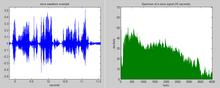
The voice waveform over time (left) has a broad audio power spectrum (right).

The power spectrum $S_{{xx}}(f)$ of a time series x(t) describes the distribution of power into frequency components composing that signal.^[1] According to Fourier analysis, any physical signal can be decomposed into a number of discrete frequencies, or a spectrum of frequencies over a continuous range. The statistical average of a certain signal or sort of signal (including noise) as analyzed in terms of its frequency content, is called its spectrum.

When the energy of the signal is concentrated around a finite time interval, especially if its total energy is finite, one may compute the energy spectral density. More commonly used is the power spectral density (or simply power spectrum), which applies to signals existing over all time, or over a time period large enough (especially in relation to the duration of a measurement) that it could as well have been over an infinite time interval. The power spectral density (PSD) then refers to the spectral energy distribution that would be found per unit time, since the total energy of such a signal over all time would generally be infinite. Summation or integration of the spectral components yields the total power (for a physical process) or variance (in a statistical process), identical to what would be obtained by integrating ${displaystyle x^{2}(t)}$ over the time domain, as dictated by Parseval’s theorem.^[1]

The spectrum of a physical process x(t) often contains essential information about the nature of . For instance, the pitch and timbre of a musical instrument are immediately determined from a spectral analysis. The color of a light source is determined by the spectrum of the electromagnetic wave’s electric field E(t) as it fluctuates at an extremely high frequency. Obtaining a spectrum from time series such as these involves the Fourier transform, and generalizations based on Fourier analysis. In many cases the time domain is not specifically employed in practice, such as when a dispersive prism is used to obtain a spectrum of light in a spectrograph, or when a sound is perceived through its effect on the auditory receptors of the inner ear, each of which is sensitive to a particular frequency.

However this article concentrates on situations in which the time series is known (at least in a statistical sense) or directly measured (such as by a microphone sampled by a computer). The power spectrum is important in statistical signal processing and in the statistical study of stochastic processes, as well as in many other branches of physics and engineering. Typically the process is a function of time, but one can similarly discuss data in the spatial domain being decomposed in terms of spatial frequency.^[1]

Units[edit]

In physics, the signal might be a wave, such as an electromagnetic wave, an acoustic wave, or the vibration of a mechanism. The power spectral density (PSD) of the signal describes the power present in the signal as a function of frequency, per unit frequency. Power spectral density is commonly expressed in watts per hertz (W/Hz).^[2]

When a signal is defined in terms only of a voltage, for instance, there is no unique power associated with the stated amplitude. In this case «power» is simply reckoned in terms of the square of the signal, as this would always be proportional to the actual power delivered by that signal into a given impedance. So one might use units of V² Hz⁻¹ for the PSD. Energy spectral density (ESD) would have units would be V² s Hz⁻¹, since energy has units of power multiplied by time (e.g., watt-hour).^[3]

In the general case, the units of PSD will be the ratio of units of variance per unit of frequency; so, for example, a series of displacement values (in meters) over time (in seconds) will have PSD in units of meters squared per hertz, m²/Hz.
In the analysis of random vibrations, units of g² Hz⁻¹ are frequently used for the PSD of acceleration, where g denotes the g-force.^[4]

Mathematically, it is not necessary to assign physical dimensions to the signal or to the independent variable. In the following discussion the meaning of x(t) will remain unspecified, but the independent variable will be assumed to be that of time.

Definition[edit]

Energy spectral density[edit]

«Energy spectral density» redirects here. Not to be confused with energy spectrum.

Energy spectral density describes how the energy of a signal or a time series is distributed with frequency. Here, the term energy is used in the generalized sense of signal processing;^[5] that is, the energy of a signal x(t) is:

${displaystyle Etriangleq int _{-infty }^{infty }left|x(t)right|^{2} dt.}$

The energy spectral density is most suitable for transients—that is, pulse-like signals—having a finite total energy. Finite or not, Parseval’s theorem^[6] (or Plancherel’s theorem) gives us an alternate expression for the energy of the signal:

${displaystyle int _{-infty }^{infty }|x(t)|^{2},dt=int _{-infty }^{infty }left|{hat {x}}(f)right|^{2} df,}$

where:

${displaystyle {hat {x}}(f)triangleq int _{-infty }^{infty }e^{-i2pi ft}x(t) dt}$

is the value of the Fourier transform of x(t) at frequency (in Hz). The theorem also holds true in the discrete-time cases. Since the integral on the left-hand side is the energy of the signal, the value of ${displaystyle left|{hat {x}}(f)right|^{2}df}$ can be interpreted as a density function multiplied by an infinitesimally small frequency interval, describing the energy contained in the signal at frequency in the frequency interval .

Therefore, the energy spectral density of x(t) is defined as:^[6]

${displaystyle {bar {S}}_{xx}(f)triangleq left|{hat {x}}(f)right|^{2}}$

(Eq.1)

The function ${displaystyle {bar {S}}_{xx}(f)}$ and the autocorrelation of x(t) form a Fourier transform pair, a result also known as the Wiener–Khinchin theorem (see also Periodogram).

As a physical example of how one might measure the energy spectral density of a signal, suppose V(t) represents the potential (in volts) of an electrical pulse propagating along a transmission line of impedance , and suppose the line is terminated with a matched resistor (so that all of the pulse energy is delivered to the resistor and none is reflected back). By Ohm’s law, the power delivered to the resistor at time is equal to $V(t)^{2}/Z$ , so the total energy is found by integrating $V(t)^{2}/Z$ with respect to time over the duration of the pulse. To find the value of the energy spectral density ${displaystyle {bar {S}}_{xx}(f)}$ at frequency , one could insert between the transmission line and the resistor a bandpass filter which passes only a narrow range of frequencies ( Delta f , say) near the frequency of interest and then measure the total energy E(f) dissipated across the resistor. The value of the energy spectral density at is then estimated to be . In this example, since the power $V(t)^{2}/Z$ has units of V² Ω⁻¹, the energy E(f) has units of V² s Ω⁻¹ = J, and hence the estimate of the energy spectral density has units of J Hz⁻¹, as required. In many situations, it is common to forget the step of dividing by so that the energy spectral density instead has units of V² Hz⁻².

This definition generalizes in a straightforward manner to a discrete signal with a countably infinite number of values $x_{n}$ such as a signal sampled at discrete times ${displaystyle t_{n}=t_{0}+(n,Delta t)}$ :

${displaystyle {bar {S}}_{xx}(f)=lim _{Nto infty }(Delta t)^{2}underbrace {left|sum _{n=-N}^{N}x_{n}e^{-i2pi fn,Delta t}right|^{2}} _{left|{hat {x}}_{d}(f)right|^{2}},}$

where ${hat {x}}_{d}(f)$ is the discrete-time Fourier transform of ${displaystyle x_{n}.}$ The sampling interval Delta t is needed to keep the correct physical units and to ensure that we recover the continuous case in the limit But in the mathematical sciences the interval is often set to 1, which simplifies the results at the expense of generality. (also see normalized frequency)

Power spectral density[edit]

The above definition of energy spectral density is suitable for transients (pulse-like signals) whose energy is concentrated around one time window; then the Fourier transforms of the signals generally exist. For continuous signals over all time, one must rather define the power spectral density (PSD) which exists for stationary processes; this describes how the power of a signal or time series is distributed over frequency, as in the simple example given previously. Here, power can be the actual physical power, or more often, for convenience with abstract signals, is simply identified with the squared value of the signal. For example, statisticians study the variance of a function over time x(t) (or over another independent variable), and using an analogy with electrical signals (among other physical processes), it is customary to refer to it as the power spectrum even when there is no physical power involved. If one were to create a physical voltage source which followed x(t) and applied it to the terminals of a one ohm resistor, then indeed the instantaneous power dissipated in that resistor would be given by ${displaystyle x(t)^{2}}$ watts.

The average power of a signal x(t) over all time is therefore given by the following time average, where the period is centered about some arbitrary time ${displaystyle t=t_{0}}$ :

${displaystyle P=lim _{Tto infty }{frac {1}{T}}int _{t_{0}-T/2}^{t_{0}+T/2}|x(t)|^{2},dt}$

However, for the sake of dealing with the math that follows, it is more convenient to deal with time limits in the signal itself rather than time limits in the bounds of the integral. As such, we have an alternative representation of the average power, where ${displaystyle x_{T}(t)=x(t)w_{T}(t)}$ and ${displaystyle w_{T}(t)}$ is unity within the arbitrary period and zero elsewhere.

${displaystyle P=lim _{Tto infty }{frac {1}{T}}int _{-infty }^{infty }|x_{T}(t)|^{2},dt}$

Clearly in cases where the above expression for P is non-zero (even as T grows without bound) the integral itself must also grow without bound. That is the reason that we cannot use the energy spectral density itself, which is that diverging integral, in such cases.

In analyzing the frequency content of the signal x(t) , one might like to compute the ordinary Fourier transform ; however, for many signals of interest the Fourier transform does not formally exist.^{[N 1]} Regardless, Parseval’s theorem tells us that we can re-write the average power as follows.

${displaystyle P=lim _{Tto infty }{frac {1}{T}}int _{-infty }^{infty }|{hat {x}}_{T}(f)|^{2},df}$

Then the power spectral density is simply defined as the integrand above.^[8]^[9]

${displaystyle S_{xx}(f)=lim _{Tto infty }{frac {1}{T}}|{hat {x}}_{T}(f)|^{2},}$

(Eq.2)

From here, we can also view ${displaystyle |{hat {x}}_{T}(f)|^{2}}$ as the Fourier transform of the time convolution of ${displaystyle x_{T}^{*}(-t)}$ and ${displaystyle x_{T}(t)}$

${displaystyle left|{hat {x}}_{T}(f)right|^{2}={mathcal {F}}left{x_{T}^{*}(-t)mathbin {mathbf {*} } x_{T}(t)right}=int _{-infty }^{infty }left[int _{-infty }^{infty }x_{T}^{*}(t-tau )x_{T}(t)dtright]e^{-i2pi ftau } dtau }$

Now, if we divide the time convolution above by the period and take the limit as , it becomes the autocorrelation function of the non-windowed signal x(t) , which is denoted as ${displaystyle R_{xx}(tau )}$ , provided that x(t) is ergodic, which is true in most, but not all, practical cases.^[10].

${displaystyle lim _{Tto infty }{frac {1}{T}}left|{hat {x}}_{T}(f)right|^{2}=int _{-infty }^{infty }left[lim _{Tto infty }{frac {1}{T}}int _{-infty }^{infty }x_{T}^{*}(t-tau )x_{T}(t)dtright]e^{-i2pi ftau } dtau =int _{-infty }^{infty }R_{xx}(tau )e^{-i2pi ftau }dtau }$

From here we see, again assuming the ergodicity of x(t) , that the power spectral density can be found as the Fourier transform of the autocorrelation function (Wiener–Khinchin theorem).

${displaystyle S_{xx}(f)=int _{-infty }^{infty }R_{xx}(tau )e^{-i2pi ftau },dtau ={hat {R}}_{xx}(f)}$

(Eq.3)

Many authors use this equality to actually define the power spectral density.^[11]

The power of the signal in a given frequency band $[f_{1},f_{2}]$ , where ${displaystyle 0<f_{1}<f_{2}}$ , can be calculated by integrating over frequency. Since ${displaystyle S_{xx}(-f)=S_{xx}(f)}$ , an equal amount of power can be attributed to positive and negative frequency bands, which accounts for the factor of 2 in the following form (such trivial factors depend on the conventions used):

${displaystyle P_{textsf {bandlimited}}=2int _{f_{1}}^{f_{2}}S_{xx}(f),df}$

More generally, similar techniques may be used to estimate a time-varying spectral density. In this case the time interval is finite rather than approaching infinity. This results in decreased spectral coverage and resolution since frequencies of less than 1/T are not sampled, and results at frequencies which are not an integer multiple of 1/T are not independent. Just using a single such time series, the estimated power spectrum will be very «noisy»; however this can be alleviated if it is possible to evaluate the expected value (in the above equation) using a large (or infinite) number of short-term spectra corresponding to statistical ensembles of realizations of x(t) evaluated over the specified time window.

Just as with the energy spectral density, the definition of the power spectral density can be generalized to discrete time variables $x_{n}$ . As before, we can consider a window of with the signal sampled at discrete times ${displaystyle x_{n}=x_{0}+(n,Delta t)}$ for a total measurement period .

${displaystyle S_{xx}(f)=lim _{Nto infty }{frac {(Delta t)^{2}}{T}}left|sum _{n=-N}^{N}x_{n}e^{-i2pi fn,Delta t}right|^{2}}$

Note that a single estimate of the PSD can be obtained through a finite number of samplings. As before, the actual PSD is achieved when (and thus ) approaches infinity and the expected value is formally applied. In a real-world application, one would typically average a finite-measurement PSD over many trials to obtain a more accurate estimate of the theoretical PSD of the physical process underlying the individual measurements. This computed PSD is sometimes called a periodogram. This periodogram converges to the true PSD as the number of estimates as well as the averaging time interval approach infinity (Brown & Hwang).^[12]

If two signals both possess power spectral densities, then the cross-spectral density can similarly be calculated; as the PSD is related to the autocorrelation, so is the cross-spectral density related to the cross-correlation.

Properties of the power spectral density[edit]

Some properties of the PSD include:^[13]

Cross power spectral density [edit]

Given two signals x(t) and y(t) , each of which possess power spectral densities $S_{{xx}}(f)$ and ${displaystyle S_{yy}(f)}$ , it is possible to define a cross power spectral density (CPSD) or cross spectral density (CSD). To begin, let us consider the average power of such a combined signal.

${displaystyle {begin{aligned}P&=lim _{Tto infty }{frac {1}{T}}int _{-infty }^{infty }left[x_{T}(t)+y_{T}(t)right]^{*}left[x_{T}(t)+y_{T}(t)right]dt\&=lim _{Tto infty }{frac {1}{T}}int _{-infty }^{infty }|x_{T}(t)|^{2}+x_{T}^{*}(t)y_{T}(t)+y_{T}^{*}(t)x_{T}(t)+|y_{T}(t)|^{2}dt\end{aligned}}}$

Using the same notation and methods as used for the power spectral density derivation, we exploit Parseval’s theorem and obtain

${displaystyle {begin{aligned}S_{xy}(f)&=lim _{Tto infty }{frac {1}{T}}left[{hat {x}}_{T}^{*}(f){hat {y}}_{T}(f)right]&S_{yx}(f)&=lim _{Tto infty }{frac {1}{T}}left[{hat {y}}_{T}^{*}(f){hat {x}}_{T}(f)right]end{aligned}}}$

where, again, the contributions of $S_{{xx}}(f)$ and ${displaystyle S_{yy}(f)}$ are already understood. Note that ${displaystyle S_{xy}^{*}(f)=S_{yx}(f)}$ , so the full contribution to the cross power is, generally, from twice the real part of either individual CPSD. Just as before, from here we recast these products as the Fourier transform of a time convolution, which when divided by the period and taken to the limit becomes the Fourier transform of a cross-correlation function.^[15]

${displaystyle {begin{aligned}S_{xy}(f)&=int _{-infty }^{infty }left[lim _{Tto infty }{frac {1}{T}}int _{-infty }^{infty }x_{T}^{*}(t-tau )y_{T}(t)dtright]e^{-i2pi ftau }dtau =int _{-infty }^{infty }R_{xy}(tau )e^{-i2pi ftau }dtau \S_{yx}(f)&=int _{-infty }^{infty }left[lim _{Tto infty }{frac {1}{T}}int _{-infty }^{infty }y_{T}^{*}(t-tau )x_{T}(t)dtright]e^{-i2pi ftau }dtau =int _{-infty }^{infty }R_{yx}(tau )e^{-i2pi ftau }dtau end{aligned}}}$

where ${displaystyle R_{xy}(tau )}$ is the cross-correlation of x(t) with y(t) and ${displaystyle R_{yx}(tau )}$ is the cross-correlation of y(t) with x(t) . In light of this, the PSD is seen to be a special case of the CSD for . If x(t) and y(t) are real signals (e.g. voltage or current), their Fourier transforms and are usually restricted to positive frequencies by convention. Therefore, in typical signal processing, the full CPSD is just one of the CPSDs scaled by a factor of two.

${displaystyle operatorname {CPSD} _{text{Full}}=2S_{xy}(f)=2S_{yx}(f)}$

For discrete signals x_n and y_n, the relationship between the cross-spectral density and the cross-covariance is

${displaystyle S_{xy}(f)=sum _{n=-infty }^{infty }R_{xy}(tau _{n})e^{-i2pi ftau _{n}},Delta tau }$

Estimation[edit]

The goal of spectral density estimation is to estimate the spectral density of a random signal from a sequence of time samples. Depending on what is known about the signal, estimation techniques can involve parametric or non-parametric approaches, and may be based on time-domain or frequency-domain analysis. For example, a common parametric technique involves fitting the observations to an autoregressive model. A common non-parametric technique is the periodogram.

The spectral density is usually estimated using Fourier transform methods (such as the Welch method), but other techniques such as the maximum entropy method can also be used.

[edit]

The spectral centroid of a signal is the midpoint of its spectral density function, i.e. the frequency that divides the distribution into two equal parts.
The spectral edge frequency (SEF), usually expressed as «SEF x«, represents the frequency below which x percent of the total power of a given signal are located; typically, x is in the range 75 to 95. It is more particularly a popular measure used in EEG monitoring, in which case SEF has variously been used to estimate the depth of anesthesia and stages of sleep.^[16]^[17]^[18]
A spectral envelope is the envelope curve of the spectrum density. It describes one point in time (one window, to be precise). For example, in remote sensing using a spectrometer, the spectral envelope of a feature is the boundary of its spectral properties, as defined by the range of brightness levels in each of the spectral bands of interest.^[19]
The spectral density is a function of frequency, not a function of time. However, the spectral density of a small window of a longer signal may be calculated, and plotted versus time associated with the window. Such a graph is called a spectrogram. This is the basis of a number of spectral analysis techniques such as the short-time Fourier transform and wavelets.
A «spectrum» generally means the power spectral density, as discussed above, which depicts the distribution of signal content over frequency. For transfer functions (e.g., Bode plot, chirp) the complete frequency response may be graphed in two parts: power versus frequency and phase versus frequency—the phase spectral density, phase spectrum, or spectral phase. Less commonly, the two parts may be the real and imaginary parts of the transfer function. This is not to be confused with the frequency response of a transfer function, which also includes a phase (or equivalently, a real and imaginary part) as a function of frequency. The time-domain impulse response cannot generally be uniquely recovered from the power spectral density alone without the phase part. Although these are also Fourier transform pairs, there is no symmetry (as there is for the autocorrelation) forcing the Fourier transform to be real-valued. See Ultrashort pulse#Spectral phase, phase noise, group delay.
Sometimes one encounters an amplitude spectral density (ASD), which is the square root of the PSD; the ASD of a voltage signal has units of V Hz^−1/2.^[20] This is useful when the shape of the spectrum is rather constant, since variations in the ASD will then be proportional to variations in the signal’s voltage level itself. But it is mathematically preferred to use the PSD, since only in that case is the area under the curve meaningful in terms of actual power over all frequency or over a specified bandwidth.

Applications[edit]

Any signal that can be represented as a variable that varies in time has a corresponding frequency spectrum. This includes familiar entities such as visible light (perceived as color), musical notes (perceived as pitch), radio/TV (specified by their frequency, or sometimes wavelength) and even the regular rotation of the earth. When these signals are viewed in the form of a frequency spectrum, certain aspects of the received signals or the underlying processes producing them are revealed. In some cases the frequency spectrum may include a distinct peak corresponding to a sine wave component. And additionally there may be peaks corresponding to harmonics of a fundamental peak, indicating a periodic signal which is not simply sinusoidal. Or a continuous spectrum may show narrow frequency intervals which are strongly enhanced corresponding to resonances, or frequency intervals containing almost zero power as would be produced by a notch filter.

Electrical engineering[edit]

Spectrogram of an FM radio signal with frequency on the horizontal axis and time increasing upwards on the vertical axis.

The concept and use of the power spectrum of a signal is fundamental in electrical engineering, especially in electronic communication systems, including radio communications, radars, and related systems, plus passive remote sensing technology. Electronic instruments called spectrum analyzers are used to observe and measure the power spectra of signals.

The spectrum analyzer measures the magnitude of the short-time Fourier transform (STFT) of an input signal. If the signal being analyzed can be considered a stationary process, the STFT is a good smoothed estimate of its power spectral density.

Cosmology[edit]

Primordial fluctuations, density variations in the early universe, are quantified by a power spectrum which gives the power of the variations as a function of spatial scale.

Climate Science[edit]

Power spectral-analysis have been used to examine the spatial structures for climate research.^[21] These results suggests atmospheric turbulence link climate change to more local regional volatility in weather conditions.^[22]

Notes[edit]

References[edit]

^ ^a ^b ^c P Stoica & R Moses (2005). «Spectral Analysis of Signals» (PDF).
^ Gérard Maral (2003). VSAT Networks. John Wiley and Sons. ISBN 978-0-470-86684-9.
^ Michael Peter Norton & Denis G. Karczub (2003). Fundamentals of Noise and Vibration Analysis for Engineers. Cambridge University Press. ISBN 978-0-521-49913-2.
^ Alessandro Birolini (2007). Reliability Engineering. Springer. p. 83. ISBN 978-3-540-49388-4.
^ Oppenheim; Verghese. Signals, Systems, and Inference. pp. 32–4.
^ ^a ^b Stein, Jonathan Y. (2000). Digital Signal Processing: A Computer Science Perspective. Wiley. p. 115.
^ Hannes Risken (1996). The Fokker–Planck Equation: Methods of Solution and Applications (2nd ed.). Springer. p. 30. ISBN 9783540615309.
^ Fred Rieke; William Bialek & David Warland (1999). Spikes: Exploring the Neural Code (Computational Neuroscience). MIT Press. ISBN 978-0262681087.
^ Scott Millers & Donald Childers (2012). Probability and random processes. Academic Press. pp. 370–5.
^ The Wiener–Khinchin theorem makes sense of this formula for any wide-sense stationary process under weaker hypotheses: $R_{{xx}}$ does not need to be absolutely integrable, it only needs to exist. But the integral can no longer be interpreted as usual. The formula also makes sense if interpreted as involving distributions (in the sense of Laurent Schwartz, not in the sense of a statistical Cumulative distribution function) instead of functions. If $R_{{xx}}$ is continuous, Bochner’s theorem can be used to prove that its Fourier transform exists as a positive measure, whose distribution function is F (but not necessarily as a function and not necessarily possessing a probability density).
^ Dennis Ward Ricker (2003). Echo Signal Processing. Springer. ISBN 978-1-4020-7395-3.
^ Robert Grover Brown & Patrick Y.C. Hwang (1997). Introduction to Random Signals and Applied Kalman Filtering. John Wiley & Sons. ISBN 978-0-471-12839-7.
^ Von Storch, H.; Zwiers, F. W. (2001). Statistical analysis in climate research. Cambridge University Press. ISBN 978-0-521-01230-0.
^ An Introduction to the Theory of Random Signals and Noise, Wilbur B. Davenport and Willian L. Root, IEEE Press, New York, 1987, ISBN 0-87942-235-1
^ William D Penny (2009). «Signal Processing Course, chapter 7».
^ Iranmanesh, Saam; Rodriguez-Villegas, Esther (2017). «An Ultralow-Power Sleep Spindle Detection System on Chip». IEEE Transactions on Biomedical Circuits and Systems. 11 (4): 858–866. doi:10.1109/TBCAS.2017.2690908. hdl:10044/1/46059. PMID 28541914. S2CID 206608057.
^ Imtiaz, Syed Anas; Rodriguez-Villegas, Esther (2014). «A Low Computational Cost Algorithm for REM Sleep Detection Using Single Channel EEG». Annals of Biomedical Engineering. 42 (11): 2344–59. doi:10.1007/s10439-014-1085-6. PMC 4204008. PMID 25113231.
^ Drummond JC, Brann CA, Perkins DE, Wolfe DE: «A comparison of median frequency, spectral edge frequency, a frequency band power ratio, total power, and dominance shift in the determination of depth of anesthesia,» Acta Anaesthesiol. Scand. 1991 Nov;35(8):693-9.
^ Swartz, Diemo (1998). «Spectral Envelopes». [1].
^ Michael Cerna & Audrey F. Harvey (2000). «The Fundamentals of FFT-Based Signal Analysis and Measurement» (PDF).
^ Communication, N. B. I. (2022-05-23). «Danish astrophysics student discovers link between global warming and locally unstable weather». nbi.ku.dk. Retrieved 2022-07-23.
^ Sneppen, Albert (2022-05-05). «The power spectrum of climate change». The European Physical Journal Plus. 137 (5): 555. arXiv:2205.07908. Bibcode:2022EPJP..137..555S. doi:10.1140/epjp/s13360-022-02773-w. ISSN 2190-5444. S2CID 248652864.

External links[edit]

Power Spectral Density Matlab scripts

Источник

1.3.1. Спектральная плотность энергии

1.3.2. Спектральная плотность мощности

Спектральная плотность (spectral density) характеристик сигнала — это распределение энергии или мощности сигнала по диапазону частот. Особую важность это понятие приобретает при рассмотрении фильтрации в системах связи. Мы должны иметь возможность оценить сигнал и шум на выходе фильтра. При проведении подобной оценки используется спектральная плотность энергии (energy spectral density — ESD) или спектральная плотность мощности (power spectral density — PSD).

1.3.1. Спектральная плотность энергии

Общая энергия действительного энергетического сигнала , определенного в интервале описывается уравнением (1.7). Используя теорему Парсеваля [1], мы можем связать энергию такого сигнала, выраженную во временной области, с энергией, выраженной в частотной области:

, (1.13)

где — Фурье-образ непериодического сигнала . (Краткие сведения об анализе Фурье можно найти в приложении А.) Обозначим через прямоугольный амплитудный спектр, определенный как

(1.14)

Величина является спектральной плотностью энергии (ESD) сигнала . Следовательно, из уравнения (1.13) можно выразить общую энергию путем интегрирования спектральной плотности по частоте.

(1.15)

Данное уравнение показывает, что энергия сигнала равна площади под на графике в частотной области. Спектральная плотность энергии описывает энергию сигнала на единицу ширины полосы и измеряется в Дж/Гц. Положительные и отрицательные частотные компоненты дают равные энергетические вклады, поэтому, для реального сигнала , величина представляет собой четную функцию частоты. Следовательно, спектральная плотность энергии симметрична по частоте относительно начала координат, а общую энергию сигнала можно выразить следующим образом.

(1.16)

1.3.2. Спектральная плотность мощности

Средняя мощность действительного сигнала в периодическом представлении определяется уравнением (1.8). Если — это периодический сигнал с периодом , он классифицируется как сигнал в периодическом представлении. Выражение для средней мощности периодического сигнала дается формулой (1.6), где среднее по времени берется за один период .

(1.17,а)

Теорема Парсеваля для действительного периодического сигнала [1] имеет вид

, (1.17,б)

где члены являются комплексными коэффициентами ряда Фурье для периодического сигнала (см. приложение А).

Чтобы использовать уравнение (1.17,6), необходимо знать только значение коэффициентов . Спектральная плотность мощности (PSD) периодического сигнала , которая является действительной, четной и неотрицательной функцией частоты и дает распределение мощности сигнала по диапазону частот, определяется следующим образом.

(1.18)

Уравнение (1.18) определяет спектральную плотность мощности периодического сигнала как последовательность взвешенных дельта-функций. Следовательно, PSD периодического сигнала является дискретной функцией частоты. Используя PSD, определенную в уравнении (1.18), можно записать среднюю нормированную мощность действительного сигнала.

(1.19)

Уравнение (1.18) описывает PSD только периодических сигналов. Если — непериодический сигнал, он не может быть выражен через ряд Фурье; если он является непериодическим сигналом в периодическом представлении (имеющим бесконечную энергию), он может не иметь Фурье-образа. Впрочем, мы по-прежнему можем выразить спектральную плотность мощности таких сигналов в пределе. Если сформировать усеченную версию непериодического сигнала в периодическом представлении , взяв для этого только его значения из интервала (), то будет иметь конечную энергию и соответствующий Фурье-образ . Можно показать [2], что спектральная плотность мощности непериодического сигнала определяется как предел.

(1.20)

Пример 1.1. Средняя нормированная мощность

а) Найдите среднюю нормированную мощность сигнала , используя усреднение по времени.

б) Выполните п. а путем суммирования спектральных коэффициентов.

Решение

а) Используя уравнение (1.17,а), имеем следующее.

б) Используя уравнения (1.18) и (1.19), получаем следующее.

(см. приложение А)

Источник

Наиболее важной
характеристикой стационарных случайных
процессов является спектральная
плотность мощности, описывающая
распределение мощности шума по частотному
спектру. Рассмотрим
стационарный случайный процесс, который
может быть представлен беспорядочной
последовательностью импульсов напряжения
или тока, следующих друг за другом через
случайные интервалы времени. Процесс
со случайной последовательностью
импульсов является непериодическим.
Тем не менее, можно говорить о спектре
такого процесса, понимая в данном случае
под спектром распределение мощности
по частотам.

Для
описания шумов вводят понятие спектральной
плотности мощности (СПМ) шума, называемой
также в общем случае спектральной
плотностью (СП) шума,которая
определяется соотношением:

(2.10)

где P(f)
— усредненная по времени мощность шума
в полосе частотfна частоте измеренияf.

Как
следует из соотношения (2.10), СП шума
имеет размерность Вт/Гц. В общем случае
СП является функцией частоты. Зависимость
СП шума от частоты называют энергетическим
спектром,
который
несет информацию о динамических
характеристиках системы.

Если
случайный процесс эргодический, то
можно находить
энергетический спектр такого процесса
по его единственной реализации, что
широко используется на практике..

При рассмотрении
спектральных характеристик стационарного
случайного процесса часто оказывается
необходимым пользоваться понятием
ширины спектра шума. Площадь под кривой
энергетического спектра случайного
процесса, отнесенную к СП шума на
некоторой характерной частоте f₀,
называютэффективной шириной спектра,
которая определяется по формуле:

(2.11)

Эту
величину можно трактовать как ширину
равномерного энергетического спектра
случайного процесса в полосе,
эквивалентного по средней мощности
рассматриваемому процессу.

Мощность шума P,
заключенная в полосе частотf₁…f₂, равна

(2.12)

Если СП шума в
полосе частот f₁…f₂постоянна и равнаS₀, тогда для
мощности шума в данной полосе частот
имеем:гдеf =f₂—f₁– полоса частот, пропускаемая
схемой или измерительным прибором.

Важным случаем
стационарного случайного процесса
является белый шум, для которого
спектральная плотность не зависит от
частоты в широком диапазоне частот
(теоретически – в бесконечном диапазоне
частот). Энергетический спектр белого
шума в диапазоне частот -∞ < f
< +∞ дается выражением:

= 2S₀
= const,
(2.13)

Модель белого шума
описывает случайный процесс без памяти
(без последействия). Белый
шумвозникает в системах с большим
числом простых однородных элементов и
характеризуется распределением амплитуды
флуктуаций по нормальному закону.
Свойства белого шума определяются
статистикой независимых одиночных
событий (например, тепловым движением
носителей заряда в проводнике или
полупроводнике). Вместе с тем истинный
белый шум с бесконечной полосой частот
не существует, поскольку он имеет
бесконечную мощность.

На рис. 2.3. приведена
типичная осциллограмма белого шума
(зависимость мгновенных значений
напряжения от времени) (рис. 2.3а) и функция
распределения вероятности мгновенных
величин напряжения e,которая является нормальным распределением
(рис. 2.3б). Заштрихованная площадь под
кривой соответствует вероятности
появления мгновенных величин напряженияe,
превышающих значениеe₁.

а)
б)

Рис. 2.3. Типичная
осциллограмма белого шума (а) и функция
распределения плотности вероятности
мгновенных величин амплитуды напряжения
шума (б).

На практике при
оценке величины шума какого-либо элемента
или п/п прибора обычно измеряют
среднеквадратичное шумовое напряжение
в единицах В²или среднеквадратичный
токв единицах А². При этом СП шума
выражают в единицах В²/Гц или
А²/Гц, а спектральные плотности
флуктуаций напряженияS_u(f)
или токаS_I(f)
вычисляются по следующим формулам:

(2.14)

где
и
– усредненные по времени шумовое
напряжение и ток в полосе частотfсоответственно. Черта сверху означает
усреднение по времени.

В практических
задачах при рассмотрении флуктуаций
различных физических величин вводят
понятие обобщенной спектральной
плотности флуктуаций. При этом СП
флуктуаций, например, для сопротивления
Rвыражается в единицах Ом²/Гц;
флуктуации магнитной индукции измеряются
в единицах Тл²/Гц, а флуктуации
частоты автогенератора – в единицах
Гц²/Гц = Гц.

При сравнении
уровней шума в линейных двухполюсниках
одного и того же типа удобно пользоваться
относительной спектральной плотностью
шума, которая определяется как

=
,
(2.15)

где u– падение
постоянного напряжения на линейном
двухполюснике.

Как видно из
выражения (2.15), относительная спектральная
плотность шума S(f)
выражается в единицах Гц^-1.

Источник

Автокорреляционная функция и спектральная плотность мощности

Автокорреляционные функции детерминированного сигнала x(t) конечной длительности, периодического сигнала и случайного сигнала определяются как (1), (2), (3) соответственно:

Автокорреляционная функция периодического и случайного сигнала имеет размерность мощности, сигнала конечной длительности – размерность энергии. Автокорреляционная функция характеризует степень взаимосвязи предыдущих и последующих значений сигнала. При τ=0 она максимальна.

Функция (4) взаимной корреляции двух разных сигналов x(t), y(t) конечной длительности характеризует степень взаимосвязи этих сигналов. Величину (5) называют интервалом корреляции. Значения сигналов, отстоящие друг от друга на интервал времени больше τ_k, являются практически взаимно независимыми

Корреляционные функции вычисляют для центрированных величин. Аналогичные функции, определенные для не центрированных величин, называются ковариационными.