#статьи
- 6 окт 2022
-

0
Стыдные вопросы о логарифмах: всё, что нужно знать программисту
Объясняем, почему не стоит бояться логарифмов и как их считать в Python.
Иллюстрация: Оля Ежак для Skillbox Media

Журналист, изучает Python. Любит разбираться в мелочах, общаться с людьми и понимать их.
Прежде чем начать обсуждение, давайте немного освежим знания и решим несколько стандартных задачек:
- Чему равен log3 81?
- А lg 2 × lb 10?
- А сумма log216 2 + log216 3?
Если вы легко прорешали все три примера в уме, не пользуясь калькулятором, — можете сразу переходить к заключительной главе. Для тех же, кто слегка подзабыл школьные годы чудесные, — буквально пять минут ликбеза.
По большому счёту, логарифм — это просто перевёрнутая степень. Рассмотрим выражение 23 = 8. В нём:
- 2 — основание степени;
- 3 — показатель степени;
- 8 — результат возведения в степень.
У возведения в степень существует два обратных выражения. В одном мы ищем основание (это извлечение корня), в другом — показатель (это логарифмирование).
Таким образом, выражение 23 = 8 можно превратить в log2 8 = 3.
Закрепляем знания: логарифм — это число, в которое нужно возвести 2 (основание степени), чтобы получить 8 (результат возведения в степень).
Форма записи неинтуитивна, и поначалу можно легко спутать основание со степенью. Чтобы избежать этого, можно использовать следующее правило:
Основание у логарифма, как и у возведения в степень, находится внизу.
Чтобы лучше запомнить структуру записи, посмотрите на эти выражения и постарайтесь понять их смысл:
- log3 9 = 2
- log4 64 = 3
- log5 625 = 4
- log7 343 = 3
- log10 100 = 2
- log2 128 = 7
- log2 0,25 = −2
- log625 125 = 0,75
В общем виде запись logAB читается так: логарифм B по основанию A.
Главная часть любого логарифма — его основание. Именно наличие общего основания у нескольких логарифмических функций позволяет проводить с ними различные операции.
Основанием натурального логарифма является число Эйлера (e) — иррациональное число, приблизительно равное 2,71828.
На всякий случай напомним, что такое иррациональные числа. Так называют числа, которые нельзя записать в виде обыкновенной дроби с целыми числителем и знаменателем. При этом знаменатель не должен быть равен нулю.
Например, 0,333… — рациональное число, потому что его можно записать как 1/3. А вот число Пи или корень из 2 — иррациональны.
Так как натуральные логарифмы часто используются, для них ввели особый способ записи: ln x — это то же самое, что loge x.
Представим кристалл, который весит 1 кг и растёт со скоростью 100% в год. Можно ожидать, что через год он будет весить 2 кг, но это не так.
Каждая новая выращенная часть начнёт растить свою собственную. Когда в кристалле будет 1,1 кг, он будет расти со скоростью 1,1 кг в год, а когда в нём будет 1,5 кг — со скоростью 1,5 кг в год. Математики подсчитали, что через год масса кристалла составит e, или ≈ 2,71828 кг.
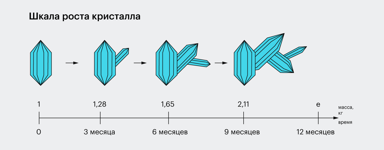
Такой рост называется экспоненциальным. По экспоненте размножаются бактерии, увеличиваются популяции, приумножаются доходы, растут снежные комья, распадается радиоактивное вещество и остывают напитки.
Чтобы узнать, какой массы достигнет кристалл через три, пять, десять лет, нужно возвести e в соответствующую степень.
e3 ≈ 20,0855 кг
e5 ≈ 148,4132 кг
e10 ≈ 22 026,4658 кг
Но как рассчитать, когда кристалл будет весить тонну? Составим уравнение:
ex = 1000
Нам известны основание степени и результат возведения в степень — осталось найти её показатель. Ничего не напоминает? Это ведь и есть логарифм x = loge 1000! Или, если использовать сокращённую запись, x = ln 1000.
Подставим в калькулятор и выясним, что x ≈ 6,9. Именно столько лет потребуется кристаллу, чтобы его масса достигла тонны.
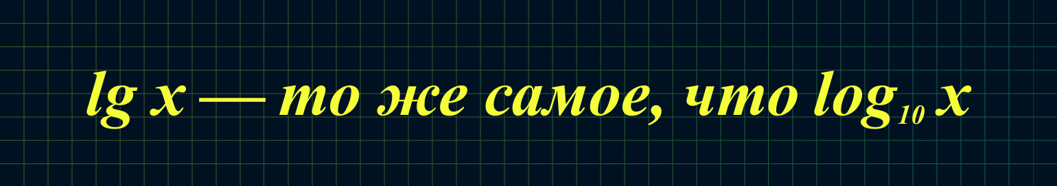
Десятичный логарифм — логарифм, основание которого равно 10. Он обозначается lg x и очень удобен, потому что с ним легко вычислять круглые числа.
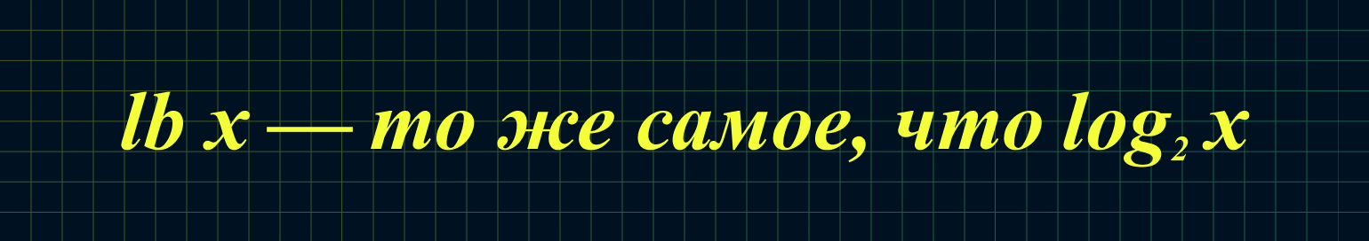
Двоичный логарифм — логарифм, основание которого равно 2. Он обозначается lb x и часто используется программистами, потому что компьютеры думают и считают в двоичной системе.
Список операций, которые можно совершать с логарифмами, ограничен. Если вы запомните все и научитесь их выполнять, то сможете щёлкать логарифмические задачки, как семечки.
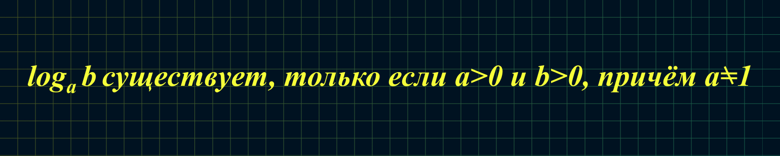
У всех логарифмов есть ограничения. Их основание и аргумент должны быть больше нуля, при этом основание не может быть равно единице. На математическом языке это звучит так:
Перейдём к свойствам логарифмов. Они работают в обе стороны, и их применяют как слева направо, так и справа налево.
1. Логарифм единицы по любому основанию всегда равен нулю:

Например: log17 1 = 0
2. Логарифм, где число и основание совпадают, равен единице:

Например: log17 17 = 1
3. Основное логарифмическое тождество:

Например: log17 175 = 5
4. Логарифм произведения чисел равен сумме их логарифмов:
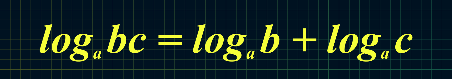
Например: log5 12,5 + log5 10 = log5 (12,5 × 10) = log5 125 = 3
5. Логарифм дроби равен разности логарифмов числителя и знаменателя:
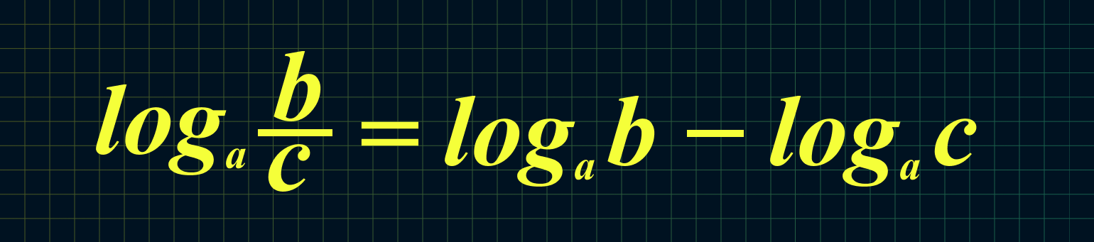
Например: log3 63 − log3 7 = log3 63/7 = log3 9 = 2
6. Если основание или аргумент возведены в степень, то их можно удобно выносить перед логарифмом:
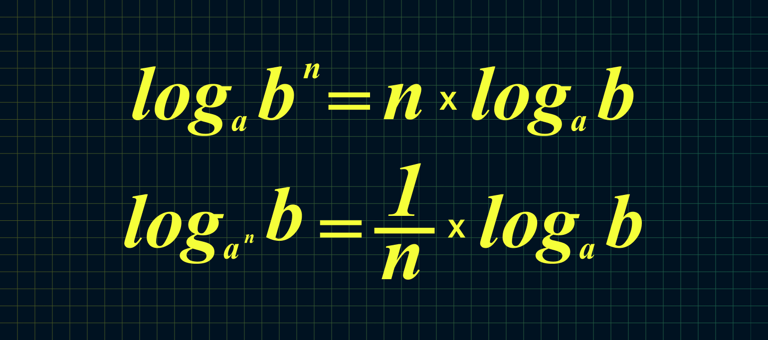
Из этих двух формул следует:
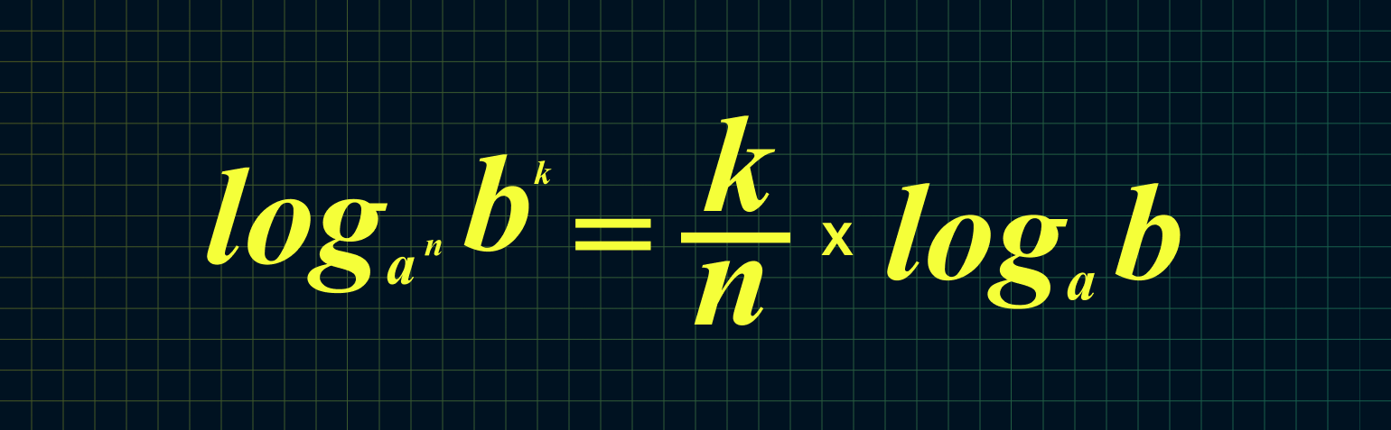
Например: log23 49 = 9/3 × log2 4 = 3 × 2 = 6
7. Если нам неудобно основание логарифма, то его можно изменить:
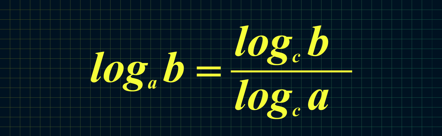
Например: log25 125 = log5 125/log5 25 = 3/2 = 1,5
Из этой формулы следует, что мы можем поменять местами основание и аргумент вот так:
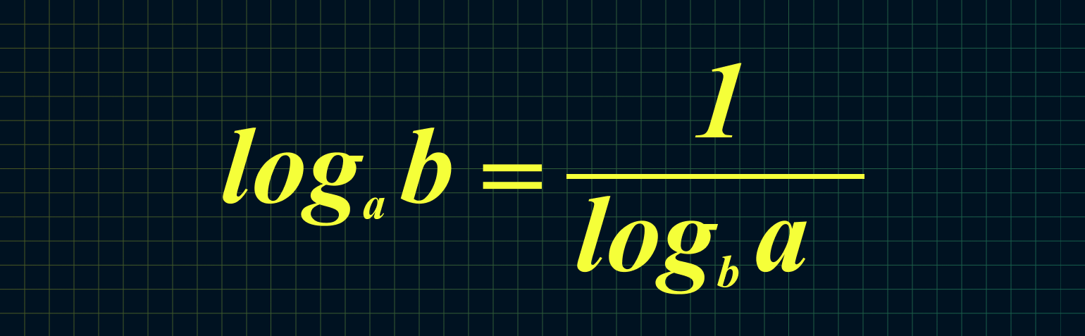
Например: log16 4 = 1/log4 16 = 1/2 = 0,5
А теперь возвращаемся к задачам, которые мы дали в начале статьи.
Пример 1
log3 81
Вспомните, что 81 — это 92. А 9 — это 32. Таким образом:
log3 81 = log3 92 = log3 32+2 = log3 34
Теперь логарифм не представляет для нас никаких сложностей. Воспользуемся свойством степени и вынесём четвёрку.
log3 34 = 4 × log3 3 = 4 × 1 =4
Ответ: 4.
Пример 2
lg 2 × lb 10
Переведём сокращённые записи в полный вид:
lg 2 × lb 10 = log10 2 × log2 10
Приведём оба логарифма к одному основанию.
log10 2 × log2 10 = 1/log2 10 × log2 10 = log2 10/log2 10 = 1
Ответ: 1.
Пример 3
log216 2 + log216 3
Воспользуемся свойством суммы.
log216 2 + log216 3 = log216 2 × 3 = log216 6
Представим 216 в виде степени числа 6 и вынесем с помощью свойства степени.
log216 6 = log63 6 = 1/3 × log6 6 = 1/3 × 1 = 1/3
Ответ: 1/3.
Чтобы работать с логарифмическими выражениями в Python, необходимо импортировать модуль math:
import math
И теперь посчитаем log2 8, используя метод math.log (b, a):
print (math.log (8, 2))
>>> 3.0
Обратите внимание на два момента. Во-первых, мы сначала передаём функции аргумент и только потом — основание. Во-вторых, функция всегда возвращает тип данных float, даже если результат целочисленный.
Если мы не передаём функции основание, то логарифм по умолчанию считается натуральным:
#math.e — метод для вызова числа Эйлера.
print (math.log (math.e))
>>> 1.0
Для подсчёта десятичного и двоичного логарифма есть отдельные методы:
#Для десятичного.
print (math.log10 (100))
>>> 2.0

#Для двоичного.
print (math.log2 (512))
>>> 9.0
Ещё в Python есть специфичный метод, который прибавляет к аргументу единицу и считает натуральный логарифм от получившегося числа:
x = math.e
print (math.log1p (x-1))
>>> 1.0
Когда х близок к нулю, этот метод даёт более точные результаты, чем math.log (1+x). Сравните:
x = 0.00001

print (math.log(x+1))
>>> 9.999950000398841e-06
print (math.log1p(x))
>>> 9.99995000033333e-06
Это все основные инструменты для работы с логарифмами в Python.
Научитесь: Профессия Python-разработчик
Узнать больше
Логарифмом положительного числа (c) по основанию (a) ((a>0, aneq1)) называется показатель степени (b), в которую надо возвести основание (a), чтобы получить число (c) ((c>0)), т.е.
(a^{b}=c) (Leftrightarrow) (log_{a}{c}=b)
Объясним проще. Например, (log_{2}{8}) равен степени, в которую надо возвести (2), чтоб получить (8). Отсюда понятно, что (log_{2}{8}=3).
|
Примеры: |
(log_{5}{25}=2) |
т.к. (5^{2}=25) |
||
|
(log_{3}{81}=4) |
т.к. (3^{4}=81) |
|||
|
(log_{2})(frac{1}{32})(=-5) |
т.к. (2^{-5}=)(frac{1}{32}) |
Аргумент и основание логарифма
Любой логарифм имеет следующую «анатомию»:

Аргумент логарифма обычно пишется на его уровне, а основание — подстрочным шрифтом ближе к знаку логарифма. А читается эта запись так: «логарифм двадцати пяти по основанию пять».
Как вычислить логарифм?
Чтобы вычислить логарифм — нужно ответить на вопрос: в какую степень следует возвести основание, чтобы получить аргумент?
Например, вычислите логарифм: а) (log_{4}{16}) б) (log_{3})(frac{1}{3}) в) (log_{sqrt{5}}{1}) г) (log_{sqrt{7}}{sqrt{7}}) д) (log_{3}{sqrt{3}})
а) В какую степень надо возвести (4), чтобы получить (16)? Очевидно во вторую. Поэтому:
(log_{4}{16}=2)
б) В какую степень надо возвести (3), чтобы получить (frac{1}{3})? В минус первую, так как именно отрицательная степень «переворачивает дробь» (здесь и далее пользуемся свойствами степени).
(log_{3})(frac{1}{3})(=-1)
в) В какую степень надо возвести (sqrt{5}), чтобы получить (1)? А какая степень делает любое число единицей? Ноль, конечно!
(log_{sqrt{5}}{1}=0)
г) В какую степень надо возвести (sqrt{7}), чтобы получить (sqrt{7})? В первую – любое число в первой степени равно самому себе.
(log_{sqrt{7}}{sqrt{7}}=1)
д) В какую степень надо возвести (3), чтобы получить (sqrt{3})? Из свойств степени мы знаем, что корень – это дробная степень, и значит квадратный корень — это степень (frac{1}{2}).
(log_{3}{sqrt{3}}=)(frac{1}{2})
Пример: Вычислить логарифм (log_{4sqrt{2}}{8})
Решение:
|
(log_{4sqrt{2}}{8}=x) |
Нам надо найти значение логарифма, обозначим его за икс. Теперь воспользуемся определением логарифма: |
|
|
((4sqrt{2})^{x}=8) |
Что связывает (4sqrt{2}) и (8)? Двойка, потому что и то, и другое число можно представить степенью двойки: |
|
|
({(2^{2}cdot2^{frac{1}{2}})}^{x}=2^{3}) |
Слева воспользуемся свойствами степени: (a^{m}cdot a^{n}=a^{m+n}) и ((a^{m})^{n}=a^{mcdot n}) |
|
|
(2^{frac{5}{2}x}=2^{3}) |
Основания равны, переходим к равенству показателей |
|
|
(frac{5x}{2})(=3) |
Умножим обе части уравнения на (frac{2}{5}) |
|
|
(x=1,2) |
Получившийся корень и есть значение логарифма |
Ответ: (log_{4sqrt{2}}{8}=1,2)

Зачем придумали логарифм?
Чтобы это понять, давайте решим уравнение: (3^{x}=9). Просто подберите (x), чтобы равенство сработало. Конечно, (x=2).
А теперь решите уравнение: (3^{x}=8).Чему равен икс? Вот в том-то и дело.
Самые догадливые скажут: «икс чуть меньше двух». А как точно записать это число? Для ответа на этот вопрос и придумали логарифм. Благодаря ему, ответ здесь можно записать как (x=log_{3}{8}).
Хочу подчеркнуть, что (log_{3}{8}), как и любой логарифм — это просто число. Да, выглядит непривычно, но зато коротко. Потому что, если бы мы захотели записать его в виде десятичной дроби, то оно выглядело бы вот так: (1,892789260714…..)
Пример: Решите уравнение (4^{5x-4}=10)
Решение:
|
(4^{5x-4}=10) |
(4^{5x-4}) и (10) никак к одному основанию не привести. Значит тут не обойтись без логарифма.
Воспользуемся определением логарифма: |
|
|
(log_{4}{10}=5x-4) |
Зеркально перевернем уравнение, чтобы икс был слева |
|
|
(5x-4=log_{4}{10}) |
Перед нами линейное уравнение. Перенесем (4) вправо. И не пугайтесь логарифма, относитесь к нему как к обычному числу. |
|
|
(5x=log_{4}{10}+4) |
Поделим уравнение на 5 |
|
|
(x=)(frac{log_{4}{10}+4}{5}) |
Вот наш корень. Да, выглядит непривычно, но ответ не выбирают. |
Ответ: (frac{log_{4}{10}+4}{5})
Десятичный и натуральный логарифмы
Как указано в определении логарифма, его основанием может быть любое положительное число, кроме единицы ((a>0, aneq1)). И среди всех возможных оснований есть два встречающихся настолько часто, что для логарифмов с ними придумали особую короткую запись:
Натуральный логарифм: логарифм, у которого основание — число Эйлера (e) (равное примерно (2,7182818…)), и записывается такой логарифм как (ln{a}).
То есть, (ln{a}) это то же самое, что и (log_{e}{a}), где (a) — некоторое число.
Десятичный логарифм: логарифм, у которого основание равно 10, записывается (lg{a}).
То есть, (lg{a}) это то же самое, что и (log_{10}{a}), где (a) — некоторое число.
Основное логарифмическое тождество
У логарифмов есть множество свойств. Одно из них носит название «Основное логарифмическое тождество» и выглядит вот так:
Это свойство вытекает напрямую из определения. Посмотрим как именно эта формула появилась.
Вспомним краткую запись определения логарифма:
если (a^{b}=c), то (log_{a}{c}=b)
То есть, (b) – это тоже самое, что (log_{a}{c}). Тогда мы можем в формуле (a^{b}=c) написать (log_{a}{c}) вместо (b). Получилось (a^{log_{a}{c}}=c) – основное логарифмическое тождество.
Остальные свойства логарифмов вы можете найти здесь. С их помощью можно упрощать и вычислять значения выражений с логарифмами, которые «в лоб» посчитать сложно.
Пример: Найдите значение выражения (36^{log_{6}{5}})
Решение:
|
(36^{log_{6}{5}}=) |
Сразу пользоваться свойством (a^{log_{a}{c}}=c) мы не можем, так как в основании степени и в основании логарифма – разные числа. Однако мы знаем, что (36=6^{2}) |
|
|
(=(6^{2})^{log_{6}{5}}=) |
Зная формулу ((a^{m})^{n}=a^{mcdot n}), а так же то, что множители можно менять местами, преобразовываем выражение |
|
|
(=6^{2cdotlog_{6}{5}}=6^{log_{6}{5}cdot2}=(6^{log_{6}{5}})^{2}=) |
Вот теперь спокойно пользуемся основным логарифмическим тождеством. |
|
|
(=5^{2}=25) |
Ответ готов. |
Ответ: (25)
Как число записать в виде логарифма?
Как уже было сказано выше – любой логарифм это просто число. Верно и обратное: любое число может быть записано как логарифм. Например, мы знаем, что (log_{2}{4}) равен двум. Тогда можно вместо двойки писать (log_{2}{4}).
Но (log_{3}{9}) тоже равен (2), значит, также можно записать (2=log_{3}{9}) . Аналогично и с (log_{5}{25}), и с (log_{9}{81}), и т.д. То есть, получается
(2=log_{2}{4}=log_{3}{9}=log_{4}{16}=log_{5}{25}=log_{6}{36}=log_{7}{49}…)
Таким образом, если нам нужно, мы можем где угодно (хоть в уравнении, хоть в выражении, хоть в неравенстве) записывать двойку как логарифм с любым основанием – просто в качестве аргумента пишем основание в квадрате.
Точно также и с тройкой – ее можно записать как (log_{2}{8}), или как (log_{3}{27}), или как (log_{4}{64})… Здесь мы как аргумент пишем основание в кубе:
(3=log_{2}{8}=log_{3}{27}=log_{4}{64}=log_{5}{125}=log_{6}{216}=log_{7}{343}…)
И с четверкой:
(4=log_{2}{16}=log_{3}{81}=log_{4}{256}=log_{5}{625}=log_{6}{1296}=log_{7}{2401}…)
И с минус единицей:
(-1=) (log_{2})(frac{1}{2})(=) (log_{3})(frac{1}{3})(=) (log_{4})(frac{1}{4})(=) (log_{5})(frac{1}{5})(=) (log_{6})(frac{1}{6})(=) (log_{7})(frac{1}{7})(…)
И с одной третьей:
(frac{1}{3})(=log_{2}{sqrt[3]{2}}=log_{3}{sqrt[3]{3}}=log_{4}{sqrt[3]{4}}=log_{5}{sqrt[3]{5}}=log_{6}{sqrt[3]{6}}=log_{7}{sqrt[3]{7}}…)
И так далее.
Любое число (a) может быть представлено как логарифм с основанием (b): (a=log_{b}{b^{a}})
Пример: Найдите значение выражения (frac{log_{2}{14}}{1+log_{2}{7}})
Решение:
|
(frac{log_{2}{14}}{1+log_{2}{7}})(=) |
Превращаем единицу в логарифм с основанием (2): (1=log_{2}{2}) |
|
|
(=)(frac{log_{2}{14}}{log_{2}{2}+log_{2}{7}})(=) |
Теперь пользуемся свойством логарифмов: |
|
|
(=)(frac{log_{2}{14}}{log_{2}{(2cdot7)}})(=)(frac{log_{2}{14}}{log_{2}{14}})(=) |
В числителе и знаменателе одинаковые числа – их можно сократить. |
|
|
(=1) |
Ответ готов. |
Ответ: (1)
Смотрите также:
Логарифмические уравнения
Логарифмические неравенства
Все знакомы, что такое степень числа (если нет, то вам сюда). В таблице приведены различные степени числа 2. Глядя на таблицу, ясно, что, например, число 32 – это 2 в пятой степени, то есть двойка, умноженная на саму себя пять раз.
Теперь при помощи этой таблицы введем понятие логарифма.
Логарифм от числа 32 по основанию 2 ((log_{2}(32))) – это в какую степень нужно возвести двойку, чтобы получить 32. Из таблицы видно, что 2 нужно возвести в пятую степень. Значит наш логарифм равен 5:
$$ log_{2}(32)=5;$$
Аналогично, глядя в таблицу получим, что:
$$log_{2}(4)=2;$$
$$log_{2}(8)=3;$$
$$log_{2}(16)=4;$$
$$log_{2}(64)=6;$$
$$log_{2}(128)=7.$$
Естественно, логарифм бывает не только по основанию 2, а по любым основаниям больших 0 и неравных 1. Можете так же создавать таблицы для разных чисел. Но, конечно, со временем вы это будете делать в уме.
Теперь дадим определение логарифма в общем виде:
Логарифмом положительного числа (b) по основанию положительно числа (a) называется степень (c), в которую нужно возвести число (a), чтобы получить (b)
$$log_{a}(b)=c;$$
$$a^{c}=b.$$
Будьте внимательны! В первое время обычно путают, что такое основание и то, что стоит под логарифмом (аргумент). Логарифм — это всегда функция, зависящая от двух переменных. Чтобы их не путать, помните определение логарифма – это степень, в которую нужно возвести основание, чтобы получить аргумент.
Но, конечно, вы часто будете сталкиваться не с такими простыми логарифмами, как в примерах с двойкой, а очень часто будет, что логарифм нельзя в уме посчитать. Действительно, что скажете про логарифм пяти по основанию два:
$$log_{2}(5)=???$$
Как его посчитать? При помощи калькулятора. Он нам покажет, что такой логарифм равен иррациональному числу:
$$log_{2}(5)=2,32192809…$$
Или логарифм шести по основанию 4:
$$log_{4}(6)= 1.2924812…$$
На уроках математики пользоваться калькулятором нельзя, поэтому на экзаменах и контрольных принято оставлять такие логарифмы в виде логарифма – не считая его, это не будет ошибкой!
Но иногда можно столкнуться с заданием, где нужно примерно оценить значение логарифма – это очень просто! Давайте для примера оценим логарифм (log_{4}(6)). Необходимо подобрать слева и справа от 6 такие ближайшие числа, логарифм от которых мы сможем посчитать, другими словами, надо найти степени 4-ки ближайшие к 6-ке:
$$ log_{4}(4) lt log_{4}(6) lt log_{4}(16);$$
$$ 1 lt log_{4}(6) lt 2. $$
Значит (log_{4}(6)) принадлежите промежутку от 1 до 2:
$$ log_{4}(6) in (1;2). $$
Как посчитать логарифм
Перед тем, как научиться считать логарифмы, нужно ввести несколько ограничений. Дело в том, что функция логарифма (log_{a}(b)) существует только при положительных значениях основания (a) и аргумента (b). И кроме этого на основание накладывается условие, что оно не должно быть равно (1).
$$ log_{a}(b) quad существует,;при quad a gt 0; ;b gt 0 ;a neq 1.$$
Почему так? Это следует из определения показательной функций. Показательная функция не может быть (0). А основание не равно (1), потому что тогда логарифм теряет смысл – ведь (1) в любой степени это будет (1).
При этих ограничениях логарифм существует.
В дальнейшем при решении различных логарифмических уравнений и неравенств вам это пригодится для ОДЗ.
Обратите внимание, что само значение логарифма может быть любым. Это же степень, а степень может быть любой – отрицательной, рациональной, иррациональной и т.д.
$$log_{3}(frac{1}{3})=-1;$$
Так как (вспоминайте определение отрицательной степени)
$$3^{-1}=frac{1}{3};$$
Теперь давайте разберем общий алгоритм вычисления логарифмов:
- Во-первых, постарайтесь представить основание и аргумент (то, что стоит под логарифмом) в виде степеней с одинаковым основанием. Параллельно с этим избавляемся от всех десятичных дробей – переводим их в обыкновенные.
- Разобраться в какую степень (x) нужно возвести основание, чтобы получить аргумент. Когда у вас там и там степени с одинаковым основанием, это сделать довольно просто.
- (x) и будет искомым значением логарифма.
Давайте разберем на примерах.
Пример 1. Посчитать логарифм (9) по основанию (3): (log_{3}(9))
- Сначала представим аргумент и основание в виде степени тройки:
$$ 3=3^1, qquad 9=3^2;$$ - Теперь надо разобраться в какую степень (x) нужно возвести (3^1), чтобы получить (3^2)
$$ (3^1)^x=3^2, $$
$$ 3^{1*x}=3^2, $$
$$ 1*x=2,$$
$$ x=2.$$ - Вот мы и решили:
$$log_{3}(9)=2.$$
Пример 2. Вычислить логарифм (frac{1}{125}) по основанию (5): (log_{5}(frac{1}{125}))
- Представим аргумент и основание в виде степени пятерки:
$$ 5=5^1, qquad frac{1}{125}=frac{1}{5^3}=5^{-3};$$ - В какую степень (x) надо возвести (5^1), чтобы получить (5^{-3}):
$$ (5^1)^x=5^{-3}, $$
$$ 5^{1*x}=5^{-3},$$
$$1*x=-3,$$
$$x=-3.$$ - Получили ответ:
$$ log_{5}(frac{1}{125})=-3.$$
Пример 3. Вычислить логарифм (4) по основанию (64): (log_{64}(4))
- Представим аргумент и основание в виде степени двойки:
$$ 64=2^6, qquad 4=2^2;$$ - В какую степень (x) надо возвести (2^6), чтобы получить (2^{2}):
$$ (2^6)^x=2^{2}, $$
$$ 2^{6*x}=2^{2},$$
$$6*x=2,$$
$$x=frac{2}{6}=frac{1}{3}.$$ - Получили ответ:
$$ log_{64}(4)=frac{1}{3}.$$
Пример 4. Вычислить логарифм (1) по основанию (8): (log_{8}(1))
- Представим аргумент и основание в виде степени двойки:
$$ 8=2^3 qquad 1=2^0;$$ - В какую степень (x) надо возвести (2^3), чтобы получить (2^{0}):
$$ (2^3)^x=2^{0}, $$
$$ 2^{3*x}=2^{0},$$
$$3*x=0,$$
$$x=frac{0}{3}=0.$$ - Получили ответ:
$$ log_{8}(1)=0.$$
Пример 5. Вычислить логарифм (15) по основанию (5): (log_{5}(15))
- Представим аргумент и основание в виде степени пятерки:
$$ 5=5^1 qquad 15= ???;$$
(15) в виде степени пятерки не представляется, поэтому этот логарифм мы не можем посчитать. У него значение будет иррациональное. Оставляем так, как есть:
$$ log_{5}(15).$$
Внимание!
Как понять, что некоторое число (a) не будет являться степенью другого числа (b). Это довольно просто – нужно разложить (a) на простые множители.
$$16=2*2*2*2=2^4,$$
(16) разложили, как произведение четырех двоек, значит (16) будет степенью двойки.
$$ 48=6*8=3*2*2*2*2,$$
Разложив (48) на простые множители, видно, что у нас есть два множителя (2) и (3), значит (48) не будет степенью.
Теперь поговорим о наиболее часто встречающихся логарифмах. Для них даже придумали специально названия – десятичный логарифм и натуральный логарифм. Давайте разбираться.
Десятичный логарифм
На самом деле, все просто. Десятичный логарифм – это любой обыкновенный логарифм, но с основанием 10. Обозначается — (lg(a)).
Пример 6
$$ log_{10}(100)= lg(100)=2;$$
$$log_{10}(1000)=lg(1000)=3;$$
$$log_{10}(10)=lg(10)=1.$$
Натуральный логарифм
Натуральным логарифмом называется логарифм по основанию (e). Обозначение — (ln(x)). Что такое (e)? Так обозначают экспоненту, число-константу, равную, примерно, (2,718281828459…). Это число известно тем, что используется в многих математических законах. Просто запомните, что логарифмы с основанием (e) часто встречаются, и поэтому им придумали специальное название – натуральный логарифм.
Пример 7
$$ log_{e}(e^2)=ln(e^2)=2;$$
$$ log_{e}(e)=ln(e)=1;$$
$$ log_{e}(e^5)=ln(e^5)=5.$$
Натуральные и десятичные логарифмы подчиняются тем же самым свойствам и правилам, что и обыкновенные логарифмы.
У логарифмов есть несколько свойств, по которым можно проводить преобразования и вычисления. Кроме этих свойств, никаких операций с логарифмами делать нельзя.
Свойства логарифмов
$$1. ; log_{a}(1)=0;$$
$$2. ; log_{a}(a)=1;$$
$$3. ; log_{a}(b*c)=log_{a}(b)+ log_{a}(c);$$
$$4. ; log_{a}(frac{b}{c})= log_{a}(b)- log_{a}(c);$$
$$5. ; log_{a}(b^m)= m*log_{a}(b);$$
$$6. ; log_{a^m}(b)=frac{1}{m}* log_{a}(b);$$
$$ 7. ; log_{a}(b)=frac{ log_{c}(b)}{ log_{c}(a)}, ; b gt 0; ; c gt 0; ; c neq 1; $$
$$ 8. ; log_{a}(b)=frac{1}{log_{b}(a)};$$
$$ 9. ; a^{ log_{a}(b)}=b.$$
Давайте разберем несколько примеров на свойства логарифмов.
Пример 8. Воспользоваться формулой (3). Логарифм от произведения – это сумма логарифмов.
$$log_{a}(b*c)=log_{a}(b)+ log_{a}(c);$$
$$ log_{3}(12)=log_{3}(3*4)=log_{3}(3)+log_{3}(4)=1+log_{3}(4);$$
$$ log_{3}(2.7)+log_{3}(10)=log_{3}(2.7*10)=log_{3}(27)=3;$$
Пример 9. Воспользоваться формулой (4). Логарифм от частного – это разность логарифмов.
$$ log_{a}(frac{b}{c})= log_{a}(b)- log_{a}(c);$$
$$ log_{7}(98)-log_{7}(2)=log_{7}(frac{98}{2})=log_{7}(49)=2;$$
Пример 10. Формула (5,6). Свойства степени.
$$log_{a}(b^m)= m*log_{a}(b);$$
$$log_{a^m}(b)=frac{1}{m}* log_{a}(b);$$
Логично, что будет выполняться и такое соотношение:
$$log_{a^m}(b^n)=frac{n}{m}* log_{a}(b);$$
И если (m=n), то:
$$log_{a^m}(b^m)=frac{m}{m}* log_{a}(b);=log_{a}(b)$$
$$log_{4}(9)=log_{2^2}(3^2)=log_{2}(3);$$
Пример 11. Формулы (7,8). Переход к другому основанию.
$$ log_{a}(b)=frac{ log_{c}(b)}{ log_{c}(a)}, ; b gt 0;c gt 0;c neq 1; $$
$$ log_{a}(b)=frac{1}{log_{b}(a)};$$
$$log_{4}(5)=frac{1}{log_{5}(4)};$$
$$log_{4}(5)=frac{log_{7}(5)}{log_{7}(4)};$$

Plots of logarithm functions, with three commonly used bases. The special points logb b = 1 are indicated by dotted lines, and all curves intersect in logb 1 = 0.
In mathematics, the logarithm is the inverse function to exponentiation. That means that the logarithm of a number x to the base b is the exponent to which b must be raised to produce x. For example, since 1000 = 103, the logarithm base 10 of 1000 is 3, or log10 (1000) = 3. The logarithm of x to base b is denoted as logb (x), or without parentheses, logb x, or even without the explicit base, log x, when no confusion is possible, or when the base does not matter such as in big O notation.
The logarithm base 10 is called the decimal or common logarithm and is commonly used in science and engineering. The natural logarithm has the number e ≈ 2.718 as its base; its use is widespread in mathematics and physics, because of its very simple derivative. The binary logarithm uses base 2 and is frequently used in computer science.
Logarithms were introduced by John Napier in 1614 as a means of simplifying calculations.[1] They were rapidly adopted by navigators, scientists, engineers, surveyors and others to perform high-accuracy computations more easily. Using logarithm tables, tedious multi-digit multiplication steps can be replaced by table look-ups and simpler addition. This is possible because the logarithm of a product is the sum of the logarithms of the factors:

provided that b, x and y are all positive and b ≠ 1. The slide rule, also based on logarithms, allows quick calculations without tables, but at lower precision. The present-day notion of logarithms comes from Leonhard Euler, who connected them to the exponential function in the 18th century, and who also introduced the letter e as the base of natural logarithms.[2]
Logarithmic scales reduce wide-ranging quantities to smaller scopes. For example, the decibel (dB) is a unit used to express ratio as logarithms, mostly for signal power and amplitude (of which sound pressure is a common example). In chemistry, pH is a logarithmic measure for the acidity of an aqueous solution. Logarithms are commonplace in scientific formulae, and in measurements of the complexity of algorithms and of geometric objects called fractals. They help to describe frequency ratios of musical intervals, appear in formulas counting prime numbers or approximating factorials, inform some models in psychophysics, and can aid in forensic accounting.
The concept of logarithm as the inverse of exponentiation extends to other mathematical structures as well. However, in general settings, the logarithm tends to be a multi-valued function. For example, the complex logarithm is the multi-valued inverse of the complex exponential function. Similarly, the discrete logarithm is the multi-valued inverse of the exponential function in finite groups; it has uses in public-key cryptography.
Motivation[edit]
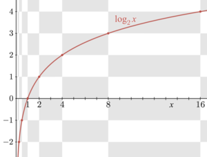
The graph of the logarithm base 2 crosses the x-axis at x = 1 and passes through the points (2, 1), (4, 2), and (8, 3), depicting, e.g., log2(8) = 3 and 23 = 8. The graph gets arbitrarily close to the y-axis, but does not meet it.
Addition, multiplication, and exponentiation are three of the most fundamental arithmetic operations. The inverse of addition is subtraction, and the inverse of multiplication is division. Similarly, a logarithm is the inverse operation of exponentiation. Exponentiation is when a number b, the base, is raised to a certain power y, the exponent, to give a value x; this is denoted

For example, raising 2 to the power of 3 gives 8: 
The logarithm of base b is the inverse operation, that provides the output y from the input x. That is,  is equivalent to
  if b is a positive real number. (If b is not a positive real number, both exponentiation and logarithm can be defined but may take several values, which makes definitions much more complicated.)
One of the main historical motivations of introducing logarithms is the formula
which allowed (before the invention of computers) reducing computation of multiplications and divisions to additions, subtractions and logarithm table looking.
Definition[edit]
Given a positive real number b such that b ≠ 1, the logarithm of a positive real number x with respect to base b[nb 1] is the exponent by which b must be raised to yield x. In other words, the logarithm of x to base b is the unique real number y such that  .[3]
.[3]
The logarithm is denoted «logb x» (pronounced as «the logarithm of x to base b«, «the base-b logarithm of x«, or most commonly «the log, base b, of x«).
An equivalent and more succinct definition is that the function logb is the inverse function to the function  .
.
Examples[edit]
Logarithmic identities[edit]
Several important formulas, sometimes called logarithmic identities or logarithmic laws, relate logarithms to one another.[4]
Product, quotient, power, and root[edit]
The logarithm of a product is the sum of the logarithms of the numbers being multiplied; the logarithm of the ratio of two numbers is the difference of the logarithms. The logarithm of the p-th power of a number is p times the logarithm of the number itself; the logarithm of a p-th root is the logarithm of the number divided by p. The following table lists these identities with examples. Each of the identities can be derived after substitution of the logarithm definitions  or
or  in the left hand sides.
| Formula | Example | |
|---|---|---|
| Product | 
|

|
| Quotient | 
|

|
| Power | 
|

|
| Root | ![{textstyle log _{b}{sqrt[{p}]{x}}={frac {log _{b}x}{p}}}](https://wikimedia.org/api/rest_v1/media/math/render/svg/68ca3b6cc8ff1c0192fb0e9206d32b14aec60e02)
|

|
Change of base[edit]
The logarithm logb x can be computed from the logarithms of x and b with respect to an arbitrary base k using the following formula:[nb 2]

Typical scientific calculators calculate the logarithms to bases 10 and e.[5] Logarithms with respect to any base b can be determined using either of these two logarithms by the previous formula:

Given a number x and its logarithm y = logb x to an unknown base b, the base is given by:

which can be seen from taking the defining equation  to the power of
Particular bases[edit]

Plots of logarithm for bases 0.5, 2, and e
Among all choices for the base, three are particularly common. These are b = 10, b = e (the irrational mathematical constant ≈ 2.71828), and b = 2 (the binary logarithm). In mathematical analysis, the logarithm base e is widespread because of analytical properties explained below. On the other hand, base-10 logarithms (the common logarithm) are easy to use for manual calculations in the decimal number system:[6]

Thus, log10 (x) is related to the number of decimal digits of a positive integer x: the number of digits is the smallest integer strictly bigger than log10 (x).[7] For example, log10(1430) is approximately 3.15. The next integer is 4, which is the number of digits of 1430. Both the natural logarithm and the binary logarithm are used in information theory, corresponding to the use of nats or bits as the fundamental units of information, respectively.[8] Binary logarithms are also used in computer science, where the binary system is ubiquitous; in music theory, where a pitch ratio of two (the octave) is ubiquitous and the number of cents between any two pitches is the binary logarithm, times 1200, of their ratio (that is, 100 cents per equal-temperament semitone); and in photography to measure exposure values, light levels, exposure times, apertures, and film speeds in «stops».[9]
The following table lists common notations for logarithms to these bases and the fields where they are used. Many disciplines write log x instead of logb x, when the intended base can be determined from the context. The «ISO notation» column lists designations suggested by the International Organization for Standardization (ISO 80000-2).[10] Because the notation log x has been used for all three bases (or when the base is indeterminate or immaterial), the intended base must often be inferred based on context or discipline. In computer science, log usually refers to log2, and in mathematics log usually refers to loge.[11] In other contexts, log often means log10.[12]
| Base b | Name for logb x | ISO notation | Other notations | Used in |
|---|---|---|---|---|
| 2 | binary logarithm | lb x[13] | ld x, log x, lg x,[14] log2 x | computer science, information theory, bioinformatics, music theory, photography |
| e | natural logarithm | ln x[nb 3] | log x (in mathematics[18] and many programming languages[nb 4]), loge x |
mathematics, physics, chemistry, statistics, economics, information theory, and engineering |
| 10 | common logarithm | lg x | log x, log10 x (in engineering, biology, astronomy) |
various engineering fields (see decibel and see below), logarithm tables, handheld calculators, spectroscopy |
| b | logarithm to base b | logb x | mathematics |
History[edit]
The history of logarithms in seventeenth-century Europe saw the discovery of a new function that extended the realm of analysis beyond the scope of algebraic methods. The method of logarithms was publicly propounded by John Napier in 1614, in a book titled Mirifici Logarithmorum Canonis Descriptio (Description of the Wonderful Canon of Logarithms).[19][20] Prior to Napier’s invention, there had been other techniques of similar scopes, such as the prosthaphaeresis or the use of tables of progressions, extensively developed by Jost Bürgi around 1600.[21][22] Napier coined the term for logarithm in Middle Latin, «logarithmus,» derived from the Greek, literally meaning, «ratio-number,» from logos «proportion, ratio, word» + arithmos «number».
The common logarithm of a number is the index of that power of ten which equals the number.[23] Speaking of a number as requiring so many figures is a rough allusion to common logarithm, and was referred to by Archimedes as the «order of a number».[24] The first real logarithms were heuristic methods to turn multiplication into addition, thus facilitating rapid computation. Some of these methods used tables derived from trigonometric identities.[25] Such methods are called prosthaphaeresis.
Invention of the function now known as the natural logarithm began as an attempt to perform a quadrature of a rectangular hyperbola by Grégoire de Saint-Vincent, a Belgian Jesuit residing in Prague. Archimedes had written The Quadrature of the Parabola in the third century BC, but a quadrature for the hyperbola eluded all efforts until Saint-Vincent published his results in 1647. The relation that the logarithm provides between a geometric progression in its argument and an arithmetic progression of values, prompted A. A. de Sarasa to make the connection of Saint-Vincent’s quadrature and the tradition of logarithms in prosthaphaeresis, leading to the term «hyperbolic logarithm», a synonym for natural logarithm. Soon the new function was appreciated by Christiaan Huygens, and James Gregory. The notation Log y was adopted by Leibniz in 1675,[26] and the next year he connected it to the integral 
Before Euler developed his modern conception of complex natural logarithms, Roger Cotes had a nearly equivalent result when he showed in 1714 that[27]
- .

Logarithm tables, slide rules, and historical applications[edit]

By simplifying difficult calculations before calculators and computers became available, logarithms contributed to the advance of science, especially astronomy. They were critical to advances in surveying, celestial navigation, and other domains. Pierre-Simon Laplace called logarithms
-
- «…[a]n admirable artifice which, by reducing to a few days the labour of many months, doubles the life of the astronomer, and spares him the errors and disgust inseparable from long calculations.»[28]
As the function f(x) = bx is the inverse function of logb x, it has been called an antilogarithm.[29] Nowadays, this function is more commonly called an exponential function.
Log tables[edit]
A key tool that enabled the practical use of logarithms was the table of logarithms.[30] The first such table was compiled by Henry Briggs in 1617, immediately after Napier’s invention but with the innovation of using 10 as the base. Briggs’ first table contained the common logarithms of all integers in the range from 1 to 1000, with a precision of 14 digits. Subsequently, tables with increasing scope were written. These tables listed the values of log10 x for any number x in a certain range, at a certain precision. Base-10 logarithms were universally used for computation, hence the name common logarithm, since numbers that differ by factors of 10 have logarithms that differ by integers. The common logarithm of x can be separated into an integer part and a fractional part, known as the characteristic and mantissa. Tables of logarithms need only include the mantissa, as the characteristic can be easily determined by counting digits from the decimal point.[31] The characteristic of 10 · x is one plus the characteristic of x, and their mantissas are the same. Thus using a three-digit log table, the logarithm of 3542 is approximated by

Greater accuracy can be obtained by interpolation:

The value of 10x can be determined by reverse look up in the same table, since the logarithm is a monotonic function.
Computations[edit]
The product and quotient of two positive numbers c and d were routinely calculated as the sum and difference of their logarithms. The product cd or quotient c/d came from looking up the antilogarithm of the sum or difference, via the same table:

and

For manual calculations that demand any appreciable precision, performing the lookups of the two logarithms, calculating their sum or difference, and looking up the antilogarithm is much faster than performing the multiplication by earlier methods such as prosthaphaeresis, which relies on trigonometric identities.
Calculations of powers and roots are reduced to multiplications or divisions and lookups by

and
![{displaystyle {sqrt[{d}]{c}}=c^{frac {1}{d}}=10^{{frac {1}{d}}log _{10}c}.}](https://wikimedia.org/api/rest_v1/media/math/render/svg/2cee4c3ee52a4b250c30c38836d4d58a006ce74c)
Trigonometric calculations were facilitated by tables that contained the common logarithms of trigonometric functions.
Slide rules[edit]
Another critical application was the slide rule, a pair of logarithmically divided scales used for calculation. The non-sliding logarithmic scale, Gunter’s rule, was invented shortly after Napier’s invention. William Oughtred enhanced it to create the slide rule—a pair of logarithmic scales movable with respect to each other. Numbers are placed on sliding scales at distances proportional to the differences between their logarithms. Sliding the upper scale appropriately amounts to mechanically adding logarithms, as illustrated here:

Schematic depiction of a slide rule. Starting from 2 on the lower scale, add the distance to 3 on the upper scale to reach the product 6. The slide rule works because it is marked such that the distance from 1 to x is proportional to the logarithm of x.
For example, adding the distance from 1 to 2 on the lower scale to the distance from 1 to 3 on the upper scale yields a product of 6, which is read off at the lower part. The slide rule was an essential calculating tool for engineers and scientists until the 1970s, because it allows, at the expense of precision, much faster computation than techniques based on tables.[32]
Analytic properties[edit]
A deeper study of logarithms requires the concept of a function. A function is a rule that, given one number, produces another number.[33] An example is the function producing the x-th power of b from any real number x, where the base b is a fixed number. This function is written as f(x) = b x. When b is positive and unequal to 1, we show below that f is invertible when considered as a function from the reals to the positive reals.
Existence[edit]
Let b be a positive real number not equal to 1 and let f(x) = b x.
It is a standard result in real analysis that any continuous strictly monotonic function is bijective between its domain and range. This fact follows from the intermediate value theorem.[34] Now, f is strictly increasing (for b > 1), or strictly decreasing (for 0 < b < 1),[35] is continuous, has domain  , and has range
  . Therefore, f is a bijection from to . In other words, for each positive real number y, there is exactly one real number x such that
  .
.
We let  denote the inverse of f. That is, logb y is the unique real number x such that . This function is called the base-b logarithm function or logarithmic function (or just logarithm).
Characterization by the product formula[edit]
The function logb x can also be essentially characterized by the product formula

More precisely, the logarithm to any base b > 1 is the only increasing function f from the positive reals to the reals satisfying f(b) = 1 and[36]

Graph of the logarithm function[edit]

The graph of the logarithm function logb (x) (blue) is obtained by reflecting the graph of the function bx (red) at the diagonal line (x = y).
As discussed above, the function logb is the inverse to the exponential function . Therefore, their graphs correspond to each other upon exchanging the x— and the y-coordinates (or upon reflection at the diagonal line x = y), as shown at the right: a point (t, u = bt) on the graph of f yields a point (u, t = logb u) on the graph of the logarithm and vice versa. As a consequence, logb (x) diverges to infinity (gets bigger than any given number) if x grows to infinity, provided that b is greater than one. In that case, logb(x) is an increasing function. For b < 1, logb (x) tends to minus infinity instead. When x approaches zero, logb x goes to minus infinity for b > 1 (plus infinity for b < 1, respectively).
Derivative and antiderivative[edit]

Analytic properties of functions pass to their inverses.[34] Thus, as f(x) = bx is a continuous and differentiable function, so is logb y. Roughly, a continuous function is differentiable if its graph has no sharp «corners». Moreover, as the derivative of f(x) evaluates to ln(b) bx by the properties of the exponential function, the chain rule implies that the derivative of logb x is given by[35][37]

That is, the slope of the tangent touching the graph of the base-b logarithm at the point (x, logb (x)) equals 1/(x ln(b)).
The derivative of ln(x) is 1/x; this implies that ln(x) is the unique antiderivative of 1/x that has the value 0 for x = 1. It is this very simple formula that motivated to qualify as «natural» the natural logarithm; this is also one of the main reasons of the importance of the constant e.
The derivative with a generalized functional argument f(x) is

The quotient at the right hand side is called the logarithmic derivative of f. Computing f’(x) by means of the derivative of ln(f(x)) is known as logarithmic differentiation.[38] The antiderivative of the natural logarithm ln(x) is:[39]

Related formulas, such as antiderivatives of logarithms to other bases can be derived from this equation using the change of bases.[40]
Integral representation of the natural logarithm[edit]

The natural logarithm of t is the shaded area underneath the graph of the function f(x) = 1/x (reciprocal of x).
The natural logarithm of t can be defined as the definite integral:

This definition has the advantage that it does not rely on the exponential function or any trigonometric functions; the definition is in terms of an integral of a simple reciprocal. As an integral, ln(t) equals the area between the x-axis and the graph of the function 1/x, ranging from x = 1 to x = t. This is a consequence of the fundamental theorem of calculus and the fact that the derivative of ln(x) is 1/x. Product and power logarithm formulas can be derived from this definition.[41] For example, the product formula ln(tu) = ln(t) + ln(u) is deduced as:

The equality (1) splits the integral into two parts, while the equality (2) is a change of variable (w = x/t). In the illustration below, the splitting corresponds to dividing the area into the yellow and blue parts. Rescaling the left hand blue area vertically by the factor t and shrinking it by the same factor horizontally does not change its size. Moving it appropriately, the area fits the graph of the function f(x) = 1/x again. Therefore, the left hand blue area, which is the integral of f(x) from t to tu is the same as the integral from 1 to u. This justifies the equality (2) with a more geometric proof.

A visual proof of the product formula of the natural logarithm
The power formula ln(tr) = r ln(t) may be derived in a similar way:

The second equality uses a change of variables (integration by substitution), w = x1/r.
The sum over the reciprocals of natural numbers,

is called the harmonic series. It is closely tied to the natural logarithm: as n tends to infinity, the difference,

converges (i.e. gets arbitrarily close) to a number known as the Euler–Mascheroni constant γ = 0.5772…. This relation aids in analyzing the performance of algorithms such as quicksort.[42]
Transcendence of the logarithm[edit]
Real numbers that are not algebraic are called transcendental;[43] for example, π and e are such numbers, but  is not. Almost all real numbers are transcendental. The logarithm is an example of a transcendental function. The Gelfond–Schneider theorem asserts that logarithms usually take transcendental, i.e. «difficult» values.[44]
Calculation[edit]
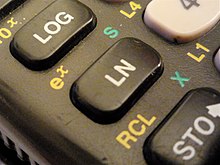
The logarithm keys (LOG for base 10 and LN for base e) on a TI-83 Plus graphing calculator
Logarithms are easy to compute in some cases, such as log10 (1000) = 3. In general, logarithms can be calculated using power series or the arithmetic–geometric mean, or be retrieved from a precalculated logarithm table that provides a fixed precision.[45][46] Newton’s method, an iterative method to solve equations approximately, can also be used to calculate the logarithm, because its inverse function, the exponential function, can be computed efficiently.[47] Using look-up tables, CORDIC-like methods can be used to compute logarithms by using only the operations of addition and bit shifts.[48][49] Moreover, the binary logarithm algorithm calculates lb(x) recursively, based on repeated squarings of x, taking advantage of the relation

Power series[edit]
Taylor series[edit]
The Taylor series of ln(z) centered at z = 1. The animation shows the first 10 approximations along with the 99th and 100th. The approximations do not converge beyond a distance of 1 from the center.
For any real number z that satisfies 0 < z ≤ 2, the following formula holds:[nb 5][50]

This is a shorthand for saying that ln(z) can be approximated to a more and more accurate value by the following expressions:

For example, with z = 1.5 the third approximation yields 0.4167, which is about 0.011 greater than ln(1.5) = 0.405465. This series approximates ln(z) with arbitrary precision, provided the number of summands is large enough. In elementary calculus, ln(z) is therefore the limit of this series. It is the Taylor series of the natural logarithm at z = 1. The Taylor series of ln(z) provides a particularly useful approximation to ln(1 + z) when z is small, |z| < 1, since then

For example, with z = 0.1 the first-order approximation gives ln(1.1) ≈ 0.1, which is less than 5% off the correct value 0.0953.
Inverse hyperbolic tangent[edit]
Another series is based on the inverse hyperbolic tangent function:

for any real number z > 0.[nb 6][50] Using sigma notation, this is also written as

This series can be derived from the above Taylor series. It converges quicker than the Taylor series, especially if z is close to 1. For example, for z = 1.5, the first three terms of the second series approximate ln(1.5) with an error of about 3×10⁻⁶. The quick convergence for z close to 1 can be taken advantage of in the following way: given a low-accuracy approximation y ≈ ln(z) and putting

the logarithm of z is:

The better the initial approximation y is, the closer A is to 1, so its logarithm can be calculated efficiently. A can be calculated using the exponential series, which converges quickly provided y is not too large. Calculating the logarithm of larger z can be reduced to smaller values of z by writing z = a · 10b, so that ln(z) = ln(a) + b · ln(10).
A closely related method can be used to compute the logarithm of integers. Putting  in the above series, it follows that:

If the logarithm of a large integer n is known, then this series yields a fast converging series for log(n+1), with a rate of convergence of  .
.
Arithmetic–geometric mean approximation[edit]
The arithmetic–geometric mean yields high precision approximations of the natural logarithm. Sasaki and Kanada showed in 1982 that it was particularly fast for precisions between 400 and 1000 decimal places, while Taylor series methods were typically faster when less precision was needed. In their work ln(x) is approximated to a precision of 2−p (or p precise bits) by the following formula (due to Carl Friedrich Gauss):[51][52]

Here M(x, y) denotes the arithmetic–geometric mean of x and y. It is obtained by repeatedly calculating the average (x + y)/2 (arithmetic mean) and  (geometric mean) of x and y then let those two numbers become the next x and y. The two numbers quickly converge to a common limit which is the value of M(x, y). m is chosen such that

to ensure the required precision. A larger m makes the M(x, y) calculation take more steps (the initial x and y are farther apart so it takes more steps to converge) but gives more precision. The constants π and ln(2) can be calculated with quickly converging series.
Feynman’s algorithm[edit]
While at Los Alamos National Laboratory working on the Manhattan Project, Richard Feynman developed a bit-processing algorithm, to compute the logarithm, that is similar to long division and was later used in the Connection Machine. The algorithm uses the fact that every real number 1 < x < 2 is representable as a product of distinct factors of the form 1 + 2−k. The algorithm sequentially builds that product P, starting with P = 1 and k = 1: if P · (1 + 2−k) < x, then it changes P to P · (1 + 2−k). It then increases  by one regardless. The algorithm stops when k is large enough to give the desired accuracy. Because log(x) is the sum of the terms of the form log(1 + 2−k) corresponding to those k for which the factor 1 + 2−k was included in the product P, log(x) may be computed by simple addition, using a table of log(1 + 2−k) for all k. Any base may be used for the logarithm table.[53]
Applications[edit]
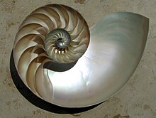
A nautilus shell displaying a logarithmic spiral
Logarithms have many applications inside and outside mathematics. Some of these occurrences are related to the notion of scale invariance. For example, each chamber of the shell of a nautilus is an approximate copy of the next one, scaled by a constant factor. This gives rise to a logarithmic spiral.[54] Benford’s law on the distribution of leading digits can also be explained by scale invariance.[55] Logarithms are also linked to self-similarity. For example, logarithms appear in the analysis of algorithms that solve a problem by dividing it into two similar smaller problems and patching their solutions.[56] The dimensions of self-similar geometric shapes, that is, shapes whose parts resemble the overall picture are also based on logarithms. Logarithmic scales are useful for quantifying the relative change of a value as opposed to its absolute difference. Moreover, because the logarithmic function log(x) grows very slowly for large x, logarithmic scales are used to compress large-scale scientific data. Logarithms also occur in numerous scientific formulas, such as the Tsiolkovsky rocket equation, the Fenske equation, or the Nernst equation.
Logarithmic scale[edit]
Scientific quantities are often expressed as logarithms of other quantities, using a logarithmic scale. For example, the decibel is a unit of measurement associated with logarithmic-scale quantities. It is based on the common logarithm of ratios—10 times the common logarithm of a power ratio or 20 times the common logarithm of a voltage ratio. It is used to quantify the loss of voltage levels in transmitting electrical signals,[57] to describe power levels of sounds in acoustics,[58] and the absorbance of light in the fields of spectrometry and optics. The signal-to-noise ratio describing the amount of unwanted noise in relation to a (meaningful) signal is also measured in decibels.[59] In a similar vein, the peak signal-to-noise ratio is commonly used to assess the quality of sound and image compression methods using the logarithm.[60]
The strength of an earthquake is measured by taking the common logarithm of the energy emitted at the quake. This is used in the moment magnitude scale or the Richter magnitude scale. For example, a 5.0 earthquake releases 32 times (101.5) and a 6.0 releases 1000 times (103) the energy of a 4.0.[61] Apparent magnitude measures the brightness of stars logarithmically.[62] In chemistry the negative of the decimal logarithm, the decimal cologarithm, is indicated by the letter p.[63] For instance, pH is the decimal cologarithm of the activity of hydronium ions (the form hydrogen ions H+
take in water).[64] The activity of hydronium ions in neutral water is 10−7 mol·L−1, hence a pH of 7. Vinegar typically has a pH of about 3. The difference of 4 corresponds to a ratio of 104 of the activity, that is, vinegar’s hydronium ion activity is about 10−3 mol·L−1.
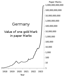
Semilog (log–linear) graphs use the logarithmic scale concept for visualization: one axis, typically the vertical one, is scaled logarithmically. For example, the chart at the right compresses the steep increase from 1 million to 1 trillion to the same space (on the vertical axis) as the increase from 1 to 1 million. In such graphs, exponential functions of the form f(x) = a · bx appear as straight lines with slope equal to the logarithm of b. Log-log graphs scale both axes logarithmically, which causes functions of the form f(x) = a · xk to be depicted as straight lines with slope equal to the exponent k. This is applied in visualizing and analyzing power laws.[65]
Psychology[edit]
Logarithms occur in several laws describing human perception:[66][67] Hick’s law proposes a logarithmic relation between the time individuals take to choose an alternative and the number of choices they have.[68] Fitts’s law predicts that the time required to rapidly move to a target area is a logarithmic function of the distance to and the size of the target.[69] In psychophysics, the Weber–Fechner law proposes a logarithmic relationship between stimulus and sensation such as the actual vs. the perceived weight of an item a person is carrying.[70] (This «law», however, is less realistic than more recent models, such as Stevens’s power law.[71])
Psychological studies found that individuals with little mathematics education tend to estimate quantities logarithmically, that is, they position a number on an unmarked line according to its logarithm, so that 10 is positioned as close to 100 as 100 is to 1000. Increasing education shifts this to a linear estimate (positioning 1000 10 times as far away) in some circumstances, while logarithms are used when the numbers to be plotted are difficult to plot linearly.[72][73]
Probability theory and statistics[edit]
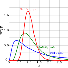
Three probability density functions (PDF) of random variables with log-normal distributions. The location parameter μ, which is zero for all three of the PDFs shown, is the mean of the logarithm of the random variable, not the mean of the variable itself.

Distribution of first digits (in %, red bars) in the population of the 237 countries of the world. Black dots indicate the distribution predicted by Benford’s law.
Logarithms arise in probability theory: the law of large numbers dictates that, for a fair coin, as the number of coin-tosses increases to infinity, the observed proportion of heads approaches one-half. The fluctuations of this proportion about one-half are described by the law of the iterated logarithm.[74]
Logarithms also occur in log-normal distributions. When the logarithm of a random variable has a normal distribution, the variable is said to have a log-normal distribution.[75] Log-normal distributions are encountered in many fields, wherever a variable is formed as the product of many independent positive random variables, for example in the study of turbulence.[76]
Logarithms are used for maximum-likelihood estimation of parametric statistical models. For such a model, the likelihood function depends on at least one parameter that must be estimated. A maximum of the likelihood function occurs at the same parameter-value as a maximum of the logarithm of the likelihood (the «log likelihood«), because the logarithm is an increasing function. The log-likelihood is easier to maximize, especially for the multiplied likelihoods for independent random variables.[77]
Benford’s law describes the occurrence of digits in many data sets, such as heights of buildings. According to Benford’s law, the probability that the first decimal-digit of an item in the data sample is d (from 1 to 9) equals log10 (d + 1) − log10 (d), regardless of the unit of measurement.[78] Thus, about 30% of the data can be expected to have 1 as first digit, 18% start with 2, etc. Auditors examine deviations from Benford’s law to detect fraudulent accounting.[79]
The logarithm transformation is a type of data transformation used to bring the empirical distribution closer to the assumed one.
Computational complexity[edit]
Analysis of algorithms is a branch of computer science that studies the performance of algorithms (computer programs solving a certain problem).[80] Logarithms are valuable for describing algorithms that divide a problem into smaller ones, and join the solutions of the subproblems.[81]
For example, to find a number in a sorted list, the binary search algorithm checks the middle entry and proceeds with the half before or after the middle entry if the number is still not found. This algorithm requires, on average, log2 (N) comparisons, where N is the list’s length.[82] Similarly, the merge sort algorithm sorts an unsorted list by dividing the list into halves and sorting these first before merging the results. Merge sort algorithms typically require a time approximately proportional to N · log(N).[83] The base of the logarithm is not specified here, because the result only changes by a constant factor when another base is used. A constant factor is usually disregarded in the analysis of algorithms under the standard uniform cost model.[84]
A function f(x) is said to grow logarithmically if f(x) is (exactly or approximately) proportional to the logarithm of x. (Biological descriptions of organism growth, however, use this term for an exponential function.[85]) For example, any natural number N can be represented in binary form in no more than log2 N + 1 bits. In other words, the amount of memory needed to store N grows logarithmically with N.
Entropy and chaos[edit]
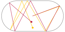
Billiards on an oval billiard table. Two particles, starting at the center with an angle differing by one degree, take paths that diverge chaotically because of reflections at the boundary.
Entropy is broadly a measure of the disorder of some system. In statistical thermodynamics, the entropy S of some physical system is defined as

The sum is over all possible states i of the system in question, such as the positions of gas particles in a container. Moreover, pi is the probability that the state i is attained and k is the Boltzmann constant. Similarly, entropy in information theory measures the quantity of information. If a message recipient may expect any one of N possible messages with equal likelihood, then the amount of information conveyed by any one such message is quantified as log2 N bits.[86]
Lyapunov exponents use logarithms to gauge the degree of chaoticity of a dynamical system. For example, for a particle moving on an oval billiard table, even small changes of the initial conditions result in very different paths of the particle. Such systems are chaotic in a deterministic way, because small measurement errors of the initial state predictably lead to largely different final states.[87] At least one Lyapunov exponent of a deterministically chaotic system is positive.
Fractals[edit]

The Sierpinski triangle (at the right) is constructed by repeatedly replacing equilateral triangles by three smaller ones.
Logarithms occur in definitions of the dimension of fractals.[88] Fractals are geometric objects that are self-similar in the sense that small parts reproduce, at least roughly, the entire global structure. The Sierpinski triangle (pictured) can be covered by three copies of itself, each having sides half the original length. This makes the Hausdorff dimension of this structure ln(3)/ln(2) ≈ 1.58. Another logarithm-based notion of dimension is obtained by counting the number of boxes needed to cover the fractal in question.
Music[edit]
![]()
![]()
Four different octaves shown on a linear scale, then shown on a logarithmic scale (as the ear hears them).
Logarithms are related to musical tones and intervals. In equal temperament, the frequency ratio depends only on the interval between two tones, not on the specific frequency, or pitch, of the individual tones. For example, the note A has a frequency of 440 Hz and B-flat has a frequency of 466 Hz. The interval between A and B-flat is a semitone, as is the one between B-flat and B (frequency 493 Hz). Accordingly, the frequency ratios agree:
![{frac {466}{440}}approx {frac {493}{466}}approx 1.059approx {sqrt[{12}]{2}}.](https://wikimedia.org/api/rest_v1/media/math/render/svg/55acf246da64ba711e1717eb43ad81792220ab32)
Therefore, logarithms can be used to describe the intervals: an interval is measured in semitones by taking the base-21/12 logarithm of the frequency ratio, while the base-21/1200 logarithm of the frequency ratio expresses the interval in cents, hundredths of a semitone. The latter is used for finer encoding, as it is needed for non-equal temperaments.[89]
| Interval (the two tones are played at the same time) |
1/12 tone |
Semitone |
Just major third |
Major third |
Tritone |
Octave |
| Frequency ratio r | 
|

|

|
![{begin{aligned}2^{frac {4}{12}}&={sqrt[{3}]{2}}\&approx 1.2599end{aligned}}](https://wikimedia.org/api/rest_v1/media/math/render/svg/76610ca7878ea438fa73bd50ac4df1fecce09b9f)
|

|

|
Corresponding number of semitones![log _{sqrt[{12}]{2}}(r)=12log _{2}(r)](https://wikimedia.org/api/rest_v1/media/math/render/svg/173477b6bc89e2396abacc83ca5015ac01b0747b)
|

|

|

|

|

|

|
Corresponding number of cents![log _{sqrt[{1200}]{2}}(r)=1200log _{2}(r)](https://wikimedia.org/api/rest_v1/media/math/render/svg/a1ccc3b05bf5ae0d41f85c50ab1a7ceec4e95713)
|

|

|

|

|

|

|
Number theory[edit]
Natural logarithms are closely linked to counting prime numbers (2, 3, 5, 7, 11, …), an important topic in number theory. For any integer x, the quantity of prime numbers less than or equal to x is denoted π(x). The prime number theorem asserts that π(x) is approximately given by

in the sense that the ratio of π(x) and that fraction approaches 1 when x tends to infinity.[90] As a consequence, the probability that a randomly chosen number between 1 and x is prime is inversely proportional to the number of decimal digits of x. A far better estimate of π(x) is given by the offset logarithmic integral function Li(x), defined by

The Riemann hypothesis, one of the oldest open mathematical conjectures, can be stated in terms of comparing π(x) and Li(x).[91] The Erdős–Kac theorem describing the number of distinct prime factors also involves the natural logarithm.
The logarithm of n factorial, n! = 1 · 2 · … · n, is given by

This can be used to obtain Stirling’s formula, an approximation of n! for large n.[92]
Generalizations[edit]
Complex logarithm[edit]
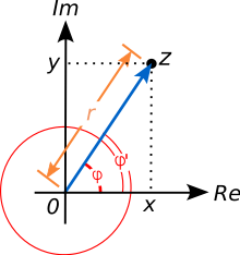
Polar form of z = x + iy. Both φ and φ’ are arguments of z.
All the complex numbers a that solve the equation

are called complex logarithms of z, when z is (considered as) a complex number. A complex number is commonly represented as z = x + iy, where x and y are real numbers and i is an imaginary unit, the square of which is −1. Such a number can be visualized by a point in the complex plane, as shown at the right. The polar form encodes a non-zero complex number z by its absolute value, that is, the (positive, real) distance r to the origin, and an angle between the real (x) axis Re and the line passing through both the origin and z. This angle is called the argument of z.
The absolute value r of z is given by

Using the geometrical interpretation of sine and cosine and their periodicity in 2π, any complex number z may be denoted as

for any integer number k. Evidently the argument of z is not uniquely specified: both φ and φ’ = φ + 2kπ are valid arguments of z for all integers k, because adding 2kπ radians or k⋅360°[nb 7] to φ corresponds to «winding» around the origin counter-clock-wise by k turns. The resulting complex number is always z, as illustrated at the right for k = 1. One may select exactly one of the possible arguments of z as the so-called principal argument, denoted Arg(z), with a capital A, by requiring φ to belong to one, conveniently selected turn, e.g. −π < φ ≤ π[93] or 0 ≤ φ < 2π.[94] These regions, where the argument of z is uniquely determined are called branches of the argument function.

The principal branch (-π, π) of the complex logarithm, Log(z). The black point at z = 1 corresponds to absolute value zero and brighter colors refer to bigger absolute values. The hue of the color encodes the argument of Log(z).
Euler’s formula connects the trigonometric functions sine and cosine to the complex exponential:

Using this formula, and again the periodicity, the following identities hold:[95]

where ln(r) is the unique real natural logarithm, ak denote the complex logarithms of z, and k is an arbitrary integer. Therefore, the complex logarithms of z, which are all those complex values ak for which the ak-th power of e equals z, are the infinitely many values
- for arbitrary integers k.

Taking k such that φ + 2kπ is within the defined interval for the principal arguments, then ak is called the principal value of the logarithm, denoted Log(z), again with a capital L. The principal argument of any positive real number x is 0; hence Log(x) is a real number and equals the real (natural) logarithm. However, the above formulas for logarithms of products and powers do not generalize to the principal value of the complex logarithm.[96]
The illustration at the right depicts Log(z), confining the arguments of z to the interval (−π, π]. This way the corresponding branch of the complex logarithm has discontinuities all along the negative real x axis, which can be seen in the jump in the hue there. This discontinuity arises from jumping to the other boundary in the same branch, when crossing a boundary, i.e. not changing to the corresponding k-value of the continuously neighboring branch. Such a locus is called a branch cut. Dropping the range restrictions on the argument makes the relations «argument of z«, and consequently the «logarithm of z«, multi-valued functions.
Inverses of other exponential functions[edit]
Exponentiation occurs in many areas of mathematics and its inverse function is often referred to as the logarithm. For example, the logarithm of a matrix is the (multi-valued) inverse function of the matrix exponential.[97] Another example is the p-adic logarithm, the inverse function of the p-adic exponential. Both are defined via Taylor series analogous to the real case.[98] In the context of differential geometry, the exponential map maps the tangent space at a point of a manifold to a neighborhood of that point. Its inverse is also called the logarithmic (or log) map.[99]
In the context of finite groups exponentiation is given by repeatedly multiplying one group element b with itself. The discrete logarithm is the integer n solving the equation

where x is an element of the group. Carrying out the exponentiation can be done efficiently, but the discrete logarithm is believed to be very hard to calculate in some groups. This asymmetry has important applications in public key cryptography, such as for example in the Diffie–Hellman key exchange, a routine that allows secure exchanges of cryptographic keys over unsecured information channels.[100] Zech’s logarithm is related to the discrete logarithm in the multiplicative group of non-zero elements of a finite field.[101]
Further logarithm-like inverse functions include the double logarithm ln(ln(x)), the super- or hyper-4-logarithm (a slight variation of which is called iterated logarithm in computer science), the Lambert W function, and the logit. They are the inverse functions of the double exponential function, tetration, of f(w) = wew,[102] and of the logistic function, respectively.[103]
[edit]
From the perspective of group theory, the identity log(cd) = log(c) + log(d) expresses a group isomorphism between positive reals under multiplication and reals under addition. Logarithmic functions are the only continuous isomorphisms between these groups.[104] By means of that isomorphism, the Haar measure (Lebesgue measure) dx on the reals corresponds to the Haar measure dx/x on the positive reals.[105] The non-negative reals not only have a multiplication, but also have addition, and form a semiring, called the probability semiring; this is in fact a semifield. The logarithm then takes multiplication to addition (log multiplication), and takes addition to log addition (LogSumExp), giving an isomorphism of semirings between the probability semiring and the log semiring.
Logarithmic one-forms df/f appear in complex analysis and algebraic geometry as differential forms with logarithmic poles.[106]
The polylogarithm is the function defined by

It is related to the natural logarithm by Li1 (z) = −ln(1 − z). Moreover, Lis (1) equals the Riemann zeta function ζ(s).[107]
See also[edit]
- Decimal exponent (dex)
- Exponential function
- Index of logarithm articles
Notes[edit]
References[edit]
- ^ Hobson, Ernest William (1914), John Napier and the invention of logarithms, 1614; a lecture, University of California Libraries, Cambridge : University Press
- ^ Remmert, Reinhold. (1991), Theory of complex functions, New York: Springer-Verlag, ISBN 0387971955, OCLC 21118309
- ^ Kate, S.K.; Bhapkar, H.R. (2009), Basics Of Mathematics, Pune: Technical Publications, ISBN 978-81-8431-755-8, chapter 1
- ^ All statements in this section can be found in Shailesh Shirali 2002, section 4, (Douglas Downing 2003, p. 275), or Kate & Bhapkar 2009, p. 1-1, for example.
- ^ Bernstein, Stephen; Bernstein, Ruth (1999), Schaum’s outline of theory and problems of elements of statistics. I, Descriptive statistics and probability, Schaum’s outline series, New York: McGraw-Hill, ISBN 978-0-07-005023-5, p. 21
- ^ Downing, Douglas (2003), Algebra the Easy Way, Barron’s Educational Series, Hauppauge, NY: Barron’s, ISBN 978-0-7641-1972-9, chapter 17, p. 275
- ^ Wegener, Ingo (2005), Complexity theory: exploring the limits of efficient algorithms, Berlin, New York: Springer-Verlag, ISBN 978-3-540-21045-0, p. 20
- ^ Van der Lubbe, Jan C. A. (1997), Information Theory, Cambridge University Press, p. 3, ISBN 978-0-521-46760-5
- ^ Allen, Elizabeth; Triantaphillidou, Sophie (2011), The Manual of Photography, Taylor & Francis, p. 228, ISBN 978-0-240-52037-7
- ^ Quantities and units – Part 2: Mathematics (ISO 80000-2:2019); EN ISO 80000-2
- ^ Goodrich, Michael T.; Tamassia, Roberto (2002), Algorithm Design: Foundations, Analysis, and Internet Examples, John Wiley & Sons, p. 23,
One of the interesting and sometimes even surprising aspects of the analysis of data structures and algorithms is the ubiquitous presence of logarithms … As is the custom in the computing literature, we omit writing the base b of the logarithm when b = 2.
- ^ Parkhurst, David F. (2007), Introduction to Applied Mathematics for Environmental Science (illustrated ed.), Springer Science & Business Media, p. 288, ISBN 978-0-387-34228-3
- ^ Gullberg, Jan (1997), Mathematics: from the birth of numbers., New York: W. W. Norton & Co, ISBN 978-0-393-04002-9
- ^ See footnote 1 in Perl, Yehoshua; Reingold, Edward M. (December 1977), «Understanding the complexity of interpolation search», Information Processing Letters, 6 (6): 219–22, doi:10.1016/0020-0190(77)90072-2
- ^
Paul Halmos (1985), I Want to Be a Mathematician: An Automathography, Berlin, New York: Springer-Verlag, ISBN 978-0-387-96078-4 - ^
Irving Stringham (1893), Uniplanar algebra: being part I of a propædeutic to the higher mathematical analysis, The Berkeley Press, p. xiii - ^
Roy S. Freedman (2006), Introduction to Financial Technology, Amsterdam: Academic Press, p. 59, ISBN 978-0-12-370478-8 - ^ See Theorem 3.29 in Rudin, Walter (1984), Principles of mathematical analysis (3rd ed., International student ed.), Auckland: McGraw-Hill International, ISBN 978-0-07-085613-4
- ^ Napier, John (1614), Mirifici Logarithmorum Canonis Descriptio [The Description of the Wonderful Canon of Logarithms] (in Latin), Edinburgh, Scotland: Andrew Hart The sequel … Constructio was published posthumously: Napier, John (1619), Mirifici Logarithmorum Canonis Constructio [The Construction of the Wonderful Rule of Logarithms] (in Latin), Edinburgh: Andrew Hart Ian Bruce has made an annotated translation of both books (2012), available from 17centurymaths.com.
- ^ Hobson, Ernest William (1914), John Napier and the invention of logarithms, 1614, Cambridge: The University Press
- ^ Folkerts, Menso; Launert, Dieter; Thom, Andreas (2016), «Jost Bürgi’s method for calculating sines», Historia Mathematica, 43 (2): 133–147, arXiv:1510.03180, doi:10.1016/j.hm.2016.03.001, MR 3489006, S2CID 119326088
- ^ O’Connor, John J.; Robertson, Edmund F., «Jost Bürgi (1552 – 1632)», MacTutor History of Mathematics archive, University of St Andrews
- ^ William Gardner (1742) Tables of Logarithms
- ^ Pierce, R. C. Jr. (January 1977), «A brief history of logarithms», The Two-Year College Mathematics Journal, 8 (1): 22–26, doi:10.2307/3026878, JSTOR 3026878
- ^ Enrique Gonzales-Velasco (2011) Journey through Mathematics – Creative Episodes in its History, §2.4 Hyperbolic logarithms, p. 117, Springer ISBN 978-0-387-92153-2
- ^ Florian Cajori (1913) «History of the exponential and logarithm concepts», American Mathematical Monthly 20: 5, 35, 75, 107, 148, 173, 205.
- ^ Stillwell, J. (2010), Mathematics and Its History (3rd ed.), Springer
- ^ Bryant, Walter W. (1907), A History of Astronomy, London: Methuen & Co, p. 44
- ^ Abramowitz, Milton; Stegun, Irene A., eds. (1972), Handbook of Mathematical Functions with Formulas, Graphs, and Mathematical Tables (10th ed.), New York: Dover Publications, ISBN 978-0-486-61272-0, section 4.7., p. 89
- ^ Campbell-Kelly, Martin (2003), The history of mathematical tables: from Sumer to spreadsheets, Oxford scholarship online, Oxford University Press, ISBN 978-0-19-850841-0, section 2
- ^ Spiegel, Murray R.; Moyer, R.E. (2006), Schaum’s outline of college algebra, Schaum’s outline series, New York: McGraw-Hill, ISBN 978-0-07-145227-4, p. 264
- ^ Maor, Eli (2009), E: The Story of a Number, Princeton University Press, sections 1, 13, ISBN 978-0-691-14134-3
- ^ Devlin, Keith (2004), Sets, functions, and logic: an introduction to abstract mathematics, Chapman & Hall/CRC mathematics (3rd ed.), Boca Raton, Fla: Chapman & Hall/CRC, ISBN 978-1-58488-449-1, or see the references in function
- ^ a b Lang, Serge (1997), Undergraduate analysis, Undergraduate Texts in Mathematics (2nd ed.), Berlin, New York: Springer-Verlag, doi:10.1007/978-1-4757-2698-5, ISBN 978-0-387-94841-6, MR 1476913, section III.3
- ^ a b Lang 1997, section IV.2
- ^ Dieudonné, Jean (1969), Foundations of Modern Analysis, vol. 1, Academic Press, p. 84 item (4.3.1)
- ^ «Calculation of d/dx(Log(b,x))«, Wolfram Alpha, Wolfram Research, retrieved 15 March 2011
- ^ Kline, Morris (1998), Calculus: an intuitive and physical approach, Dover books on mathematics, New York: Dover Publications, ISBN 978-0-486-40453-0, p. 386
- ^ «Calculation of Integrate(ln(x))«, Wolfram Alpha, Wolfram Research, retrieved 15 March 2011
- ^ Abramowitz & Stegun, eds. 1972, p. 69
- ^ Courant, Richard (1988), Differential and integral calculus. Vol. I, Wiley Classics Library, New York: John Wiley & Sons, ISBN 978-0-471-60842-4, MR 1009558, section III.6
- ^ Havil, Julian (2003), Gamma: Exploring Euler’s Constant, Princeton University Press, ISBN 978-0-691-09983-5, sections 11.5 and 13.8
- ^ Nomizu, Katsumi (1996), Selected papers on number theory and algebraic geometry, vol. 172, Providence, RI: AMS Bookstore, p. 21, ISBN 978-0-8218-0445-2
- ^ Baker, Alan (1975), Transcendental number theory, Cambridge University Press, ISBN 978-0-521-20461-3, p. 10
- ^ Muller, Jean-Michel (2006), Elementary functions (2nd ed.), Boston, MA: Birkhäuser Boston, ISBN 978-0-8176-4372-0, sections 4.2.2 (p. 72) and 5.5.2 (p. 95)
- ^ Hart; Cheney; Lawson; et al. (1968), Computer Approximations, SIAM Series in Applied Mathematics, New York: John Wiley, section 6.3, pp. 105–11
- ^ Zhang, M.; Delgado-Frias, J.G.; Vassiliadis, S. (1994), «Table driven Newton scheme for high precision logarithm generation», IEE Proceedings — Computers and Digital Techniques, 141 (5): 281–92, doi:10.1049/ip-cdt:19941268, ISSN 1350-2387, section 1 for an overview
- ^ Meggitt, J.E. (April 1962), «Pseudo Division and Pseudo Multiplication Processes», IBM Journal of Research and Development, 6 (2): 210–26, doi:10.1147/rd.62.0210, S2CID 19387286
- ^ Kahan, W. (20 May 2001), Pseudo-Division Algorithms for Floating-Point Logarithms and Exponentials
- ^ a b Abramowitz & Stegun, eds. 1972, p. 68
- ^ Sasaki, T.; Kanada, Y. (1982), «Practically fast multiple-precision evaluation of log(x)», Journal of Information Processing, 5 (4): 247–50, retrieved 30 March 2011
- ^ Ahrendt, Timm (1999), «Fast Computations of the Exponential Function», Stacs 99, Lecture notes in computer science, vol. 1564, Berlin, New York: Springer, pp. 302–12, doi:10.1007/3-540-49116-3_28, ISBN 978-3-540-65691-3
- ^ Hillis, Danny (15 January 1989), «Richard Feynman and The Connection Machine», Physics Today, 42 (2): 78, Bibcode:1989PhT….42b..78H, doi:10.1063/1.881196
- ^ Maor 2009, p. 135
- ^ Frey, Bruce (2006), Statistics hacks, Hacks Series, Sebastopol, CA: O’Reilly, ISBN 978-0-596-10164-0, chapter 6, section 64
- ^ Ricciardi, Luigi M. (1990), Lectures in applied mathematics and informatics, Manchester: Manchester University Press, ISBN 978-0-7190-2671-3, p. 21, section 1.3.2
- ^ Bakshi, U.A. (2009), Telecommunication Engineering, Pune: Technical Publications, ISBN 978-81-8431-725-1, section 5.2
- ^ Maling, George C. (2007), «Noise», in Rossing, Thomas D. (ed.), Springer handbook of acoustics, Berlin, New York: Springer-Verlag, ISBN 978-0-387-30446-5, section 23.0.2
- ^ Tashev, Ivan Jelev (2009), Sound Capture and Processing: Practical Approaches, New York: John Wiley & Sons, p. 98, ISBN 978-0-470-31983-3
- ^ Chui, C.K. (1997), Wavelets: a mathematical tool for signal processing, SIAM monographs on mathematical modeling and computation, Philadelphia: Society for Industrial and Applied Mathematics, ISBN 978-0-89871-384-8
- ^ Crauder, Bruce; Evans, Benny; Noell, Alan (2008), Functions and Change: A Modeling Approach to College Algebra (4th ed.), Boston: Cengage Learning, ISBN 978-0-547-15669-9, section 4.4.
- ^ Bradt, Hale (2004), Astronomy methods: a physical approach to astronomical observations, Cambridge Planetary Science, Cambridge University Press, ISBN 978-0-521-53551-9, section 8.3, p. 231
- ^ Nørby, Jens (2000). «The origin and the meaning of the little p in pH». Trends in Biochemical Sciences. 25 (1): 36–37. doi:10.1016/S0968-0004(99)01517-0. PMID 10637613.
- ^ IUPAC (1997), A. D. McNaught, A. Wilkinson (ed.), Compendium of Chemical Terminology («Gold Book») (2nd ed.), Oxford: Blackwell Scientific Publications, doi:10.1351/goldbook, ISBN 978-0-9678550-9-7
- ^ Bird, J.O. (2001), Newnes engineering mathematics pocket book (3rd ed.), Oxford: Newnes, ISBN 978-0-7506-4992-6, section 34
- ^ Goldstein, E. Bruce (2009), Encyclopedia of Perception, Encyclopedia of Perception, Thousand Oaks, CA: Sage, ISBN 978-1-4129-4081-8, pp. 355–56
- ^ Matthews, Gerald (2000), Human Performance: Cognition, Stress, and Individual Differences, Hove: Psychology Press, ISBN 978-0-415-04406-6, p. 48
- ^ Welford, A.T. (1968), Fundamentals of skill, London: Methuen, ISBN 978-0-416-03000-6, OCLC 219156, p. 61
- ^ Paul M. Fitts (June 1954), «The information capacity of the human motor system in controlling the amplitude of movement», Journal of Experimental Psychology, 47 (6): 381–91, doi:10.1037/h0055392, PMID 13174710, S2CID 501599, reprinted in Paul M. Fitts (1992), «The information capacity of the human motor system in controlling the amplitude of movement» (PDF), Journal of Experimental Psychology: General, 121 (3): 262–69, doi:10.1037/0096-3445.121.3.262, PMID 1402698, retrieved 30 March 2011
- ^ Banerjee, J.C. (1994), Encyclopaedic dictionary of psychological terms, New Delhi: M.D. Publications, p. 304, ISBN 978-81-85880-28-0, OCLC 33860167
- ^ Nadel, Lynn (2005), Encyclopedia of cognitive science, New York: John Wiley & Sons, ISBN 978-0-470-01619-0, lemmas Psychophysics and Perception: Overview
- ^
Siegler, Robert S.; Opfer, John E. (2003), «The Development of Numerical Estimation. Evidence for Multiple Representations of Numerical Quantity» (PDF), Psychological Science, 14 (3): 237–43, CiteSeerX 10.1.1.727.3696, doi:10.1111/1467-9280.02438, PMID 12741747, S2CID 9583202, archived from the original (PDF) on 17 May 2011, retrieved 7 January 2011 - ^ Dehaene, Stanislas; Izard, Véronique; Spelke, Elizabeth; Pica, Pierre (2008), «Log or Linear? Distinct Intuitions of the Number Scale in Western and Amazonian Indigene Cultures», Science, 320 (5880): 1217–20, Bibcode:2008Sci…320.1217D, CiteSeerX 10.1.1.362.2390, doi:10.1126/science.1156540, PMC 2610411, PMID 18511690
- ^ Breiman, Leo (1992), Probability, Classics in applied mathematics, Philadelphia: Society for Industrial and Applied Mathematics, ISBN 978-0-89871-296-4, section 12.9
- ^ Aitchison, J.; Brown, J.A.C. (1969), The lognormal distribution, Cambridge University Press, ISBN 978-0-521-04011-2, OCLC 301100935
- ^
Jean Mathieu and Julian Scott (2000), An introduction to turbulent flow, Cambridge University Press, p. 50, ISBN 978-0-521-77538-0 - ^ Rose, Colin; Smith, Murray D. (2002), Mathematical statistics with Mathematica, Springer texts in statistics, Berlin, New York: Springer-Verlag, ISBN 978-0-387-95234-5, section 11.3
- ^ Tabachnikov, Serge (2005), Geometry and Billiards, Providence, RI: American Mathematical Society, pp. 36–40, ISBN 978-0-8218-3919-5, section 2.1
- ^ Durtschi, Cindy; Hillison, William; Pacini, Carl (2004), «The Effective Use of Benford’s Law in Detecting Fraud in Accounting Data» (PDF), Journal of Forensic Accounting, V: 17–34, archived from the original (PDF) on 29 August 2017, retrieved 28 May 2018
- ^ Wegener, Ingo (2005), Complexity theory: exploring the limits of efficient algorithms, Berlin, New York: Springer-Verlag, ISBN 978-3-540-21045-0, pp. 1–2
- ^ Harel, David; Feldman, Yishai A. (2004), Algorithmics: the spirit of computing, New York: Addison-Wesley, ISBN 978-0-321-11784-7, p. 143
- ^ Knuth, Donald (1998), The Art of Computer Programming, Reading, MA: Addison-Wesley, ISBN 978-0-201-89685-5, section 6.2.1, pp. 409–26
- ^ Donald Knuth 1998, section 5.2.4, pp. 158–68
- ^ Wegener, Ingo (2005), Complexity theory: exploring the limits of efficient algorithms, Berlin, New York: Springer-Verlag, p. 20, ISBN 978-3-540-21045-0
- ^ Mohr, Hans; Schopfer, Peter (1995), Plant physiology, Berlin, New York: Springer-Verlag, ISBN 978-3-540-58016-4, chapter 19, p. 298
- ^ Eco, Umberto (1989), The open work, Harvard University Press, ISBN 978-0-674-63976-8, section III.I
- ^ Sprott, Julien Clinton (2010), «Elegant Chaos: Algebraically Simple Chaotic Flows», Elegant Chaos: Algebraically Simple Chaotic Flows. Edited by Sprott Julien Clinton. Published by World Scientific Publishing Co. Pte. Ltd, New Jersey: World Scientific, Bibcode:2010ecas.book…..S, doi:10.1142/7183, ISBN 978-981-283-881-0, section 1.9
- ^ Helmberg, Gilbert (2007), Getting acquainted with fractals, De Gruyter Textbook, Berlin, New York: Walter de Gruyter, ISBN 978-3-11-019092-2
- ^ Wright, David (2009), Mathematics and music, Providence, RI: AMS Bookstore, ISBN 978-0-8218-4873-9, chapter 5
- ^ Bateman, P.T.; Diamond, Harold G. (2004), Analytic number theory: an introductory course, New Jersey: World Scientific, ISBN 978-981-256-080-3, OCLC 492669517, theorem 4.1
- ^ P. T. Bateman & Diamond 2004, Theorem 8.15
- ^ Slomson, Alan B. (1991), An introduction to combinatorics, London: CRC Press, ISBN 978-0-412-35370-3, chapter 4
- ^ Ganguly, S. (2005), Elements of Complex Analysis, Kolkata: Academic Publishers, ISBN 978-81-87504-86-3, Definition 1.6.3
- ^ Nevanlinna, Rolf Herman; Paatero, Veikko (2007), «Introduction to complex analysis», London: Hilger, Providence, RI: AMS Bookstore, Bibcode:1974aitc.book…..W, ISBN 978-0-8218-4399-4, section 5.9
- ^ Moore, Theral Orvis; Hadlock, Edwin H. (1991), Complex analysis, Singapore: World Scientific, ISBN 978-981-02-0246-0, section 1.2
- ^ Wilde, Ivan Francis (2006), Lecture notes on complex analysis, London: Imperial College Press, ISBN 978-1-86094-642-4, theorem 6.1.
- ^ Higham, Nicholas (2008), Functions of Matrices. Theory and Computation, Philadelphia, PA: SIAM, ISBN 978-0-89871-646-7, chapter 11.
- ^ Neukirch, Jürgen (1999), Algebraische Zahlentheorie, Grundlehren der mathematischen Wissenschaften, vol. 322, Berlin: Springer-Verlag, ISBN 978-3-540-65399-8, MR 1697859, Zbl 0956.11021, section II.5.
- ^ Hancock, Edwin R.; Martin, Ralph R.; Sabin, Malcolm A. (2009), Mathematics of Surfaces XIII: 13th IMA International Conference York, UK, September 7–9, 2009 Proceedings, Springer, p. 379, ISBN 978-3-642-03595-1
- ^ Stinson, Douglas Robert (2006), Cryptography: Theory and Practice (3rd ed.), London: CRC Press, ISBN 978-1-58488-508-5
- ^ Lidl, Rudolf; Niederreiter, Harald (1997), Finite fields, Cambridge University Press, ISBN 978-0-521-39231-0
- ^ Corless, R.; Gonnet, G.; Hare, D.; Jeffrey, D.; Knuth, Donald (1996), «On the Lambert W function» (PDF), Advances in Computational Mathematics, 5: 329–59, doi:10.1007/BF02124750, ISSN 1019-7168, S2CID 29028411, archived from the original (PDF) on 14 December 2010, retrieved 13 February 2011
- ^ Cherkassky, Vladimir; Cherkassky, Vladimir S.; Mulier, Filip (2007), Learning from data: concepts, theory, and methods, Wiley series on adaptive and learning systems for signal processing, communications, and control, New York: John Wiley & Sons, ISBN 978-0-471-68182-3, p. 357
- ^ Bourbaki, Nicolas (1998), General topology. Chapters 5–10, Elements of Mathematics, Berlin, New York: Springer-Verlag, ISBN 978-3-540-64563-4, MR 1726872, section V.4.1
- ^ Ambartzumian, R.V. (1990), Factorization calculus and geometric probability, Cambridge University Press, ISBN 978-0-521-34535-4, section 1.4
- ^ Esnault, Hélène; Viehweg, Eckart (1992), Lectures on vanishing theorems, DMV Seminar, vol. 20, Basel, Boston: Birkhäuser Verlag, CiteSeerX 10.1.1.178.3227, doi:10.1007/978-3-0348-8600-0, ISBN 978-3-7643-2822-1, MR 1193913, section 2
- ^ Apostol, T.M. (2010), «Logarithm», in Olver, Frank W. J.; Lozier, Daniel M.; Boisvert, Ronald F.; Clark, Charles W. (eds.), NIST Handbook of Mathematical Functions, Cambridge University Press, ISBN 978-0-521-19225-5, MR 2723248
External links[edit]
 Media related to Logarithm at Wikimedia Commons
 The dictionary definition of logarithm at Wiktionary
 A lesson on logarithms can be found on Wikiversity
- Weisstein, Eric W., «Logarithm», MathWorld
- Khan Academy: Logarithms, free online micro lectures
- «Logarithmic function», Encyclopedia of Mathematics, EMS Press, 2001 [1994]
- Colin Byfleet, Educational video on logarithms, retrieved 12 October 2010
- Edward Wright, Translation of Napier’s work on logarithms, archived from the original on 3 December 2002, retrieved 12 October 2010
{{citation}}: CS1 maint: unfit URL (link) - Glaisher, James Whitbread Lee (1911), «Logarithm» , in Chisholm, Hugh (ed.), Encyclopædia Britannica, vol. 16 (11th ed.), Cambridge University Press, pp. 868–77
Содержание:
Множеством (областью) значений показательной функции 

Такое значение аргумента единственное, так как если  и
и  то по следствию из п. 2.3 верно равенство c = d. Это единственное значение аргумента с называют логарифмом числа b по основанию a и обозначают
  т. е.
т. е.
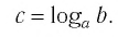
Таким образом, равенство  означает, что
  Сформулируем определение логарифма еще раз.
Определение:
Пусть  Логарифмом числа b по основанию а называется показатель степени, в которую нужно возвести число а, чтобы получить число b.
Приведем несколько примеров:
Нахождение логарифма числа называется логарифмированием.
Обозначим  Тогда, согласно определению логарифма, верно равенство
  т. е.
т. е.
Это равенство называется основным логарифмическим тождеством.
Согласно этому тождеству, например, имеем:  Основное логарифмическое тождество позволяет данное число b представить в виде степени с любым положительным основанием.
Например: 
История логарифма
Логарифмы были изобретены в 1614 г. шотландским математиком Д. Непером (1550—1617) и независимо от него на 6 лет позднее швейцарским механиком и математиком И. Бюрги (1552—1632).
Оба исследователя хотели найти новое удобное средство арифметических вычислений, но их определения логарифма различны и у обоих не похожи на современные. Понимание логарифма как показателя степени с данным основанием впервые появилось в XVIII в. в работах английского математика В. Гардинера (1742). Широкому распространению этого определения логарифма более других содействовал Jl. Эйлер, который впервые применил в этой связи и термин «основание».
Термин «логарифм» принадлежит Неперу. Он возник из сочетания греческих слов логос — отношение и аритмос — число. Слово «логарифм», таким образом, означало «число отношения».
Пример:
а) Записать число  в виде логарифмов по основанию
б) Записать число -5 в виде логарифмов по основанию  и х
и х 
Решение:
а) По определению логарифма имеем:
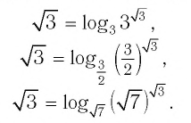
б) По определению логарифма имеем:
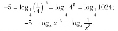
Пример:
Между какими целыми числами находится число
Решение:
Пусть  тогда верно равенство
  Поскольку
  По свойствам показательной функции с основанием 2 имеем
  Значит,
 находится между числами 4 и 5.
Ответ: 
Пример:
Решить уравнение:
Решение:
а) Поскольку  то по определению логарифма имеем
б)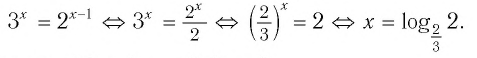
Ответ: 
Логарифмы по основанию 10 имеют особое название — десятичные логарифмы. Десятичный логарифм числа b обозначается  . Таким образом,
▲ Особое обозначение и название имеют не только десятичные логарифмы, но и логарифмы, основанием которых является число е:
Такие логарифмы называются натуральными.
Логарифмы по основанию е позволяют выражать математическую зависимость, которая характеризует многие биологические, химические, физические, социальные и другие процессы. По-видимому, этим объясняется и название «натуральные логарифмы», т. е. естественные (этот термин ввел в 1659 г. итальянский математик П. Менголи). Натуральные и десятичные логарифмы имели большое значение для облегчения вычислений в XVII—XX вв. до создания мощных современных вычислительных средств. Натуральные логарифмы имеют и большое теоретическое значение.▲
Основные свойства логарифмов
Теорема:
При любых положительных значениях b и с верно равенство:
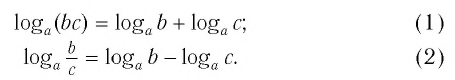
Доказательство:
Докажем утверждение (1).
По основному логарифмическому тождеству
 по свойствам степени
Таким образом, имеем:
Отсюда по следствию из п. 2.3 получаем равенство (1).
Докажем утверждение (2). Преобразуем левую часть равенства (2):
 I используя равенство (1), получим
Заметим, что равенство (2) можно доказать тем же способом, что и равенство (1), — сделайте это самостоятельно.
Равенство (1) означает, что логарифм произведения двух положительных чисел равен сумме логарифмов этих чисел.
Равенство (2) означает, что логарифм дроби с положительными. числителем и знаменателем равен разности логарифмов числителя и знаменателя.
Замечание. Равенства, доказанные в теореме 1 (как и другие равенства этого пункта), являются тождествами. Действительно, каждое из них превращается в верное числовое равенство при любых значениях a, b и с, для которых входящие в равенство выражения имеют смысл.
Теорема:
При любых значениях s и положительных значениях b верно равенство

Доказательство:
По основному логарифмическому тождеству
 по свойствам степени
Таким образом, имеем
Отсюда по следствию из п. 2.3 получаем равенство (3).
Следствие 1. Если числа  одного знака, то имеет место равенство

Следствие 2. При любом целом  имеет место равенство
Пример №1
Найти значение выражения:

Решение:
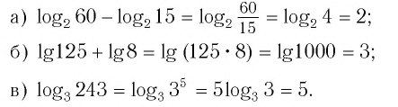
Ответ: 
Теорема:
При любых значениях  и
и  верно равенство
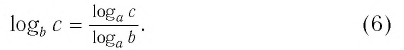
Доказательство:
Способ 1. По основному логарифмическому тождеству имеем
Прологарифмировав левую и правую части этого тождества по основанию а, получим
Применив тождество (3), имеем
Так как  Поэтому левую и правую части этого равенства можно разделить на
  В результате получим тождество (6).
Способ 2. Пусть  тогда
тогда  Логарифмируя обе части этого равенства по основанию а, получаем
Откуда имеем
Итак, 
Тождество (6) называется формулой перехода от логарифма по одному основанию к логарифму по другому основанию.
Обычно в таблицах, калькуляторах даются значения логарифмов по основанию 10, а когда нужно найти значение логарифма по другому основанию, пользуются формулой перехода от логарифма по одному основанию к логарифму по другому основанию.
Следствием из тождества (6) при основании а = с является формула
(убедитесь в этом самостоятельно).
Пример №2
Найти значение выражения, если 
Решение:
 согласно тождеству (6) имеем
используя тождество (3), получим
используя тождество (1), имеем
с учетом условия  получим
6)
на основании тождеств (6) и (7) получим
по тождеству (3) и с учетом условия имеем
Ответ: 
Следствие 3. Имеют место тождества:
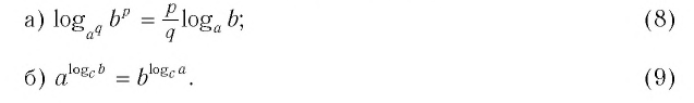
Тождества (8) и (9) можно доказать, используя уже доказанные тождества из этого пункта.
Пример №3
Упростить выражение 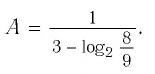
Решение:
Используя определение логарифма, представим числа 1 и 3 в виде логарифмов по основанию 2:
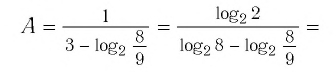
 по свойству (2) логарифмов имеем
воспользовавшись формулой (7), получим

Ответ: 
Развитие науки, прежде всего астрономии, уже в XVI в. привело к необходимости громоздких вычислений при умножении и делении многозначных чисел. Эти вычислительные проблемы были в некоторой степени решены с открытием логарифмов и созданием таблиц логарифмов.
Логарифмическая функция
Рассмотрим выражение  где х — переменная, а — постоянная,
  Это выражение имеет смысл при любом значении х > 0 и не имеет смысла при любом значении
  Таким образом, естественной областью определения выражения
 является множество всех положительных действительных чисел, т. е. промежуток
Определение:
Логарифмической функцией называется функция вида  где а — постоянная,
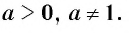
Область определения логарифмической функции — это естественная область определения выражения  т.е. множество
Графики некоторых логарифмических функций изображены на рисунке 34. Эти изображения (как и для графиков других функций) можно было получить, строя их по точкам. Отметим некоторые особенности изображенных графиков.
График функции  расположен справа от оси Оу и пересекает ось Ох в точке (1; 0).
Когда значения аргумента х уменьшаются, т. е. приближаются к нулю, то график этой функции «приближается» к оси Оу и при этом «круто» опускается вниз. А когда значения аргумента х увеличиваются, то график «медленно» поднимается вверх (ем. рис. 34). Аналогично для любой функции  при а > 1 (рис. 35). График функции
  расположен справа от оси Оу и пересекает ось Ох в точке (1; 0) (см. рис. 34).
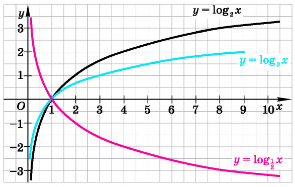

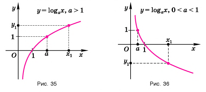
Заметим, что когда значения аргумента х уменьшаются, т. е. приближаются к нулю, то график этой функции «приближается» к оси Оу и при этом «круто» поднимается вверх. А когда значения аргумента х увеличиваются, то график «медленно» опускается вниз. Аналогично для любой функции  при 0 < а < 1 (рис. 36).
Теорема (о свойствах логарифмической функции  )
)
- Областью определения логарифмической функции является интервал
- Множеством (областью) значений логарифмической функции является множество R всех действительных чисел.
- Логарифмическая функция не имеет ни наименьшего, ни наибольшего значений.
- График логарифмической функции пересекается с осью абсцисс в точке (1; 0) и не пересекается с осью ординат.
- Значение аргумента х = 1 является нулем логарифмической функции.
- 6. При а > 1 логарифмическая функция принимает отрицательные значения на интервале (0; 1) и принимает положительные значения на интервале И при 0 < а < 1 логарифмическая функция принимает отрицательные значения на интервале и принимает положительные значения на интервале (0; 1).
- Логарифмическая функция не является ни четной, ни нечетной.
- При а > 1 логарифмическая функция возрастает на всей области определения. При 0 < а < 1 логарифмическая функция убывает на всей области определения.
- Логарифмическая функция не является периодической.

 И при 0 < а < 1 логарифмическая функция принимает отрицательные значения на интервале
  и принимает положительные значения на интервале (0; 1).
Изображение графика логарифмической функции позволяет наглядно представить эти свойства.
Множество (область) значений логарифмической функции — проекция ее графика на ось Оу, а на рисунках 35 и 36 видно, что эта проекция есть ось Оу. Это значит, что для любой точки  лежащей на оси Оу, найдется такая точка
  принадлежащая интервалу
  (свойство 2).
Множество (область) значений логарифмической функции — это множество всех действительных чисел, а в нем нет ни наименьшего числа, ни наибольшего (свойство 3).
График логарифмической функции проходит через точку (1; 0) и лежит в правой полуплоскости (свойства 4, 5).
При а > 1 график логарифмической функции лежит в IV координатном угле, когда  и лежит в I координатном угле, когда
  При 0 < а < 1 график логарифмической функции лежит в I координатном угле, когда
  и лежит в IV координатном угле, когда
 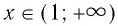 (свойство 6).
Область определения логарифмической функции — интервал  поэтому логарифмическая функция не является ни четной, ни нечетной, ни периодической (свойства 7, 9).
На рисунке 35 видно, что при а > 1 логарифмическая функция возрастает на области определения, а на рисунке 36 видно, что при 0 < а < 1 логарифмическая функция убывает на области определения (свойство 8).
Пусть точка  лежит на графике функции
  Это значит, что верно числовое равенство
 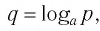 следовательно, согласно определению логарифма верно числовое равенство
  В свою очередь, последнее равенство означает, что точка
  лежит на графике функции
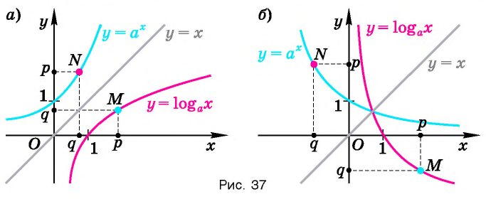
Заметим, что точки 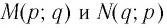 симметричны относительно прямой
  Таким образом, каждой точке М на графике функции
  соответствует симметричная ей относительно этой прямой точка N на графике функции
  и наоборот. Следовательно, графики функций
 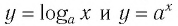 симметричны относительно прямой у = х (рис. 37).
Последнее утверждение дает возможность, зная график функции  изобразить график функции
  (не используя построение по точкам).
▲ Симметричность графиков функций 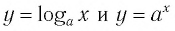 относительно прямой у=х означает, что эти функции взаимно обратны.
Функции 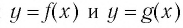 называются взаимно обратными, если для любого
  верно равенство
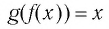 и для любого
  верно равенство
Покажем, что показательная и логарифмическая функции с одним, и тем же основанием а взаимно обратны.
Пусть  Тогда
Тогда 
Для любого 

Для любого 
Покажем, что графики взаимно обратных функций  симметричны относительно прямой у = х.
Пусть точка  лежит на графике функции
  Это означает, что верно числовое равенство
  Тогда по определению взаимно обратных функций
  А равенство
  означает, что точка
  лежит на графике функции
Таким образом, каждой точке М на графике функции  соответствует симметричная относительно прямой у = х точка N на графике функции
  и наоборот. Следовательно, графики функций
  симметричны относительно прямой
- Заказать решение задач по высшей математике
Логарифмы и их свойства
В предыдущем параграфе вы находили корни уравнения вида  Например:
  А какой корень имеет уравнение
  Графическим методом можно убедиться, что оно имеет единственное решение (рис. 28). Это число больше 2 и меньше 3, но как его записать?
Для записи корней показательного уравнения используют понятие «логарифм» и соответствующий символ. Корнем уравнения  является число, которое записывают в виде
  и читают «логарифм числа 5 по основанию 2».
Рассмотрим общий случай-.
Пусть  — действительные числа;
 Если
Если  то число
  называют логарифмом числа
  по основанию
Логарифмом числа  по основанию
  называют показатель степени, в которую нужно возвести число
  чтобы получить
Логарифм числа  по основанию
  обозначают символом
Примеры:
 так как
 так как
  так как
Основанием логарифма может быть произвольное положительное число, кроме единицы. Как известно, если  то область определения показательной функции
  — множество всех действительных чисел
  а область значений — множество всех положительных действительных чисел. Поэтому при таких значениях
  для любого положительного числа
  найдётся такое
  что
что  Другими словами: при любом основании
  где
где  существует логарифм каждого положительного числа. Логарифм отрицательного числа и нуля не существует.
Полезно помнить, что для каждого 
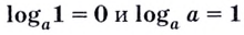 (почему?).
Нахождение логарифма числа называют логарифмированием. Эта операция обратная к операции возведения в степень с соответствующим основанием.
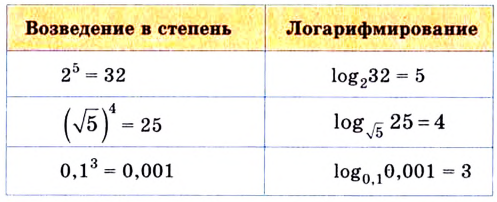
Согласно определению логарифма, если  Это разные записи одной зависимости. Из них следует равенство
которое называют основным логарифмическим тождеством. Оно правильное для любых положительных 
Например: 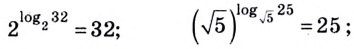
С помощью основного логарифмического тождества любое положительное число можно представить в виде степени, имеющей заданное основание.
Например: 
Докажем ещё несколько важных свойств логарифмов (для положительных 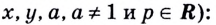
1) По основному логарифмическому тождеству и основному свойству степени

Итак, 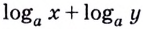 — показатель, в который нужно возвести число
  чтобы получить
  то есть
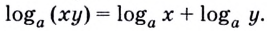
Эту формулу можно обобщить на три и более множителя:

Кратко говорят: логарифм произведения равен сумме логарифмов множителей.
2) Доказательство аналогичное предыдущему:
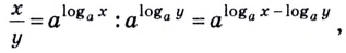
отсюда
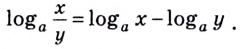
Кратко говорят: логарифм частного равен разности логарифмов делимого и делителя.
3) Возведём обе части тождества  в степень
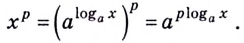
Итак,
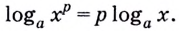
Доказанные формулы можно использовать и справа налево, например:
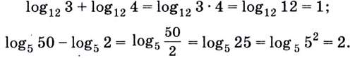
В логарифмах переходить от одного основания к другому можно при помощи формулы перехода
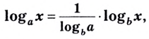
где 
Докажем эту формулу. Поскольку положительные числа  и
и  равны, то равны и их логарифмы по основанию
  Поэтому
 откуда и следует доказываемая формула.
Обратите внимание! Как следствия из формулы перехода можно получить следующие формулы:
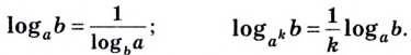
Докажите их самостоятельно.
Пример №4
Упростите выражение 
Решение:
Сведём все логарифмы к основанию 5. Имеем:
Особенно часто используют логарифмы по основаниям 10 и  их называют десятичными и натуральными логарифмами. Вместо
  пишут соответственно
Рассмотренные в параграфе свойства логарифмов правиль-1 ные при условии, что переменные принимают положительные значения. С помощью модуля можно расширить использование некоторых формул. Например:
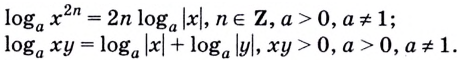
Для преобразования выражений, решения уравнений и неравенств используют и другие формулы, содержащие логарифмы:
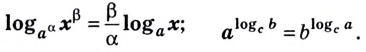
Докажите их самостоятельно.
Пример №5
Вычислите: 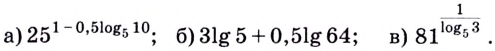
Решение:
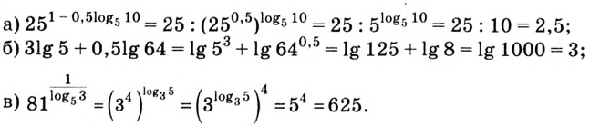
Пример №6
Решите уравнение: 
Решение:
Пусть  тогда
тогда  Подставим
  в данное уравнение.
Получим:  отсюда
Поскольку  или
или 
Ответ. 
Пример №7
Найдите  из равенства:

Решение:

Поскольку 
Ответ. 
Пример №8
Вычислите  если
если 
Решение:
Ответ. 
- Корень из числа — нахождение и вычисление
- Теория множеств — виды, операции и примеры
- Числовые множества
- Вектор — определение и основные понятия
- Бесконечно убывающая геометрическая прогрессия
- Периодические дроби
- Степень с рациональным показателем
- Степень с действительным показателем