Improve Article
Save Article
Like Article
Improve Article
Save Article
Like Article
In Python, math module contains a number of mathematical operations, which can be performed with ease using the module. math.cos() function returns the cosine of value passed as argument. The value passed in this function should be in radians.
Syntax: math.cos(x)
Parameter:
x : value to be passed to cos()Returns: Returns the cosine of value passed as argument
Code #1:
import math
a = math.pi / 6
print ("The value of cosine of pi / 6 is : ", end ="")
print (math.cos(a))
Output:
The value of cosine of pi/6 is : 0.8660254037844387
Code #2:
import math
import numpy as np
import matplotlib.pyplot as plt
in_array = np.linspace(-(2 * np.pi), 2 * np.pi, 20)
out_array = []
for i in range(len(in_array)):
out_array.append(math.cos(in_array[i]))
i += 1
print("in_array : ", in_array)
print("nout_array : ", out_array)
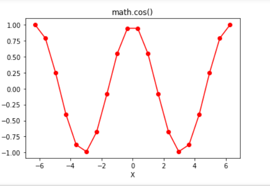
plt.plot(in_array, out_array, color = 'red', marker = "o")
plt.title("math.cos()")
plt.xlabel("X")
plt.ylabel("Y")
plt.show()
Output:
in_array : [-6.28318531 -5.62179738 -4.96040945 -4.29902153 -3.6376336 -2.97624567
-2.31485774 -1.65346982 -0.99208189 -0.33069396 0.33069396 0.99208189
1.65346982 2.31485774 2.97624567 3.6376336 4.29902153 4.96040945
5.62179738 6.28318531]out_array : [1.0, 0.7891405093963934, 0.2454854871407988, -0.40169542465296987, -0.8794737512064891, -0.9863613034027223, -0.6772815716257412, -0.08257934547233249, 0.5469481581224268, 0.9458172417006346, 0.9458172417006346, 0.5469481581224268, -0.0825793454723316, -0.6772815716257405, -0.9863613034027223, -0.8794737512064893, -0.40169542465296987, 0.2454854871407988, 0.7891405093963934, 1.0]
Last Updated :
20 Mar, 2019
Like Article
Save Article
В этом разделе представлены тригонометрические функции модуля math.
Содержание:
- Функция
math.sin(); - Функция
math.cos(); - Функция
math.tan(); - Функция
math.asin(); - Функция
math.acos(); - Функция
math.atan(); - Функция
math.atan2(); - Функция
math.hypot().
math.sin(x):
Функция math.sin() возвращает синус угла x значение которого задано в радианах.
>>> from math import *
>>> sin(pi/2)
# 1.0
>>> sin(pi/4)
# 0.7071067811865475)
math.cos(x):
Функция math.cos() возвращает косинус угла x значение которого задано в радианах.
>>> from math import *
>>> cos(pi/3)
# 0.5000000000000001
>>> cos(pi)
# -1.0
math.tan(x):
Функция math.tan() возвращает тангенс угла x значение которого задано в радианах.
>>>from math import *
>>> tan(pi/3)
# 1.7320508075688767
>>> tan(pi/4)
# 0.9999999999999999
При определенных значениях углов тангенс должен быть равен либо −∞ либо +∞, скажем tan(3π/2)=+∞, a tan(−π/2)=−∞, но вместо этого мы получаем либо очень большие либо очень маленькие значения типа float:
>>> tan(-pi/2)
# -1.633123935319537e+16
>>> tan(3*pi/2)    #  должно быть Inf, но
# 5443746451065123.0
math.asin(x):
Функция math.asin() возвращает арксинус значения x, т. е. такое значение угла y, выраженного в радианах при котором sin(y) = x.
>>> from math import *
>>> asin(sin(pi/6))
# 0.5235987755982988
>>> pi/6
# 0.5235987755982988
math.acos(x):
Функция math.acos() возвращает арккосинус значения x, т. е. возвращает такое значение угла y, выраженного в радианах, при котором cos(y) = x.
>>> from math import *
>>> acos(cos(pi/6))
0.5235987755982987
>>> pi/6
0.5235987755982988
math.atan(x):
Функция math.atan() возвращает арктангенс значения x, т. е. возвращает такое значение угла y, выраженного в радианах, при котором tan(y) = x.
>>> from math import *
>>> atan(tan(pi/6))
# 0.5235987755982988
>>> pi/6
# 0.5235987755982988
math.atan2(y, x):
Функция math.atan2() возвращает арктангенс значения y/x, т. е. возвращает такое значение угла z, выраженного в радианах, при котором tan(z) = x. Результат находится между -pi и pi.
>>> from math import *
>>> y = 1
>>> x = 2
>>> atan2(y, x)
# 0.4636476090008061
>>> atan(y/x)
# 0.4636476090008061
>>> tan(0.4636476090008061)
# 0.49999999999999994
Данная функция, в отличие от функции math.atan(), способна вычислить правильный квадрант в котором должно находиться значение результата. Это возможно благодаря тому, что функция принимает два аргумента (x, y) координаты точки, которая является концом отрезка начатого в начале координат. Сам по себе, угол между этим отрезком и положительным направлением оси X не несет информации о том где располагается конец этого отрезка, что приводит к одинаковому значению арктангенса, для разных отрезков, но функция math.atan2() позволяет избежать этого, что бывает очень важно в целом ряде задач. Например, atan(1) и atan2(1, 1) оба имеют значение pi/4, но atan2(-1, -1) равно -3 * pi / 4.
math.hypot(*coordinates):
Функция math.hypot() возвращает евклидову норму, sqrt(sum(x**2 for x in coordinates)). Это длина вектора от начала координат до точки, заданной координатами.
Для двумерной точки (x, y) это эквивалентно вычислению гипотенузы прямоугольного треугольника с использованием теоремы Пифагора sqrt(x*x + y*y).
Изменено в Python 3.8: Добавлена поддержка n-мерных точек. Раньше поддерживался только двумерный случай.
В этом уроке мы собираемся обсудить тригонометрическую функцию косинуса(cos) в Python. Мы поговорим о модулях, которые мы можем использовать для реализации функции cos в нашей программе Python. Мы также узнаем о построении графиков с помощью функции cos в программе. Итак, давайте начнем с рассмотрения модулей, которые мы можем импортировать в программу для использования функции cos.
В Python у нас есть математический модуль, который мы можем использовать для импорта и реализации функции cos, а также других важных математических операций в программе.
Помимо математического модуля, мы также можем использовать модуль numpy Python для реализации функции cos в программе. Мы изучим использование обоих модулей, т. е. модуля math и модуля numpy.
Метод 1: функция cos() в модуле math
Математический модуль Python содержит ряд важных математических значений и операций, и функция cos() является одной из них. Мы можем использовать функцию cos() модуля math для реализации тригонометрического значения cos в программе.
Функция math.cos() возвращает значение тригонометрического косинуса для аргумента, который мы указываем внутри функции, т. е. значение степени в косинусе. Значение, которое мы даем в качестве аргумента функции, должно быть в радианах.
Ниже приведен синтаксис использования функции math.cos() в программе Python:
math.cos(a)
Параметры: Здесь параметр a = значение в радианах.
Возвращаемое значение: функция math.cos() возвращает значение косинуса для аргумента ‘a’ в радианах, которое мы указали внутри функции.
Давайте разберемся с использованием функции cos() модуля math в Python с помощью следующего примера программы:
# Import math module
import math
# Define an input radian value
x = math.pi / 12
# Printing cosine value for respective input value
print("The cosine value of pi / 12 value as given is : ", end ="")

print(math.cos(x))
Выход:
The cosine value of pi / 12 value as given is: 0.9659258262890683
Метод 2: функция cos() в модуле Numpy
Помимо математического модуля, мы также можем использовать модуль numpy для реализации значения тригонометрического косинуса в программе. Для этого нам предоставляется функция cos() внутри модуля numpy, которая дает нам математическое значение косинуса на выходе.
Как и функция math.cos(), при использовании функции cos() модуля numpy мы должны указать значение аргумента в радианах внутри функции.
Ниже приведен синтаксис использования функции numpy.cos() в программе Python:
numpy.cos(a)
Параметры: мы можем указать ‘a’ в качестве следующих типов параметров внутри функции numpy.cos():
- В функции можно указать аргумент с одним значением в радианах.
- Мы также можем предоставить массив, содержащий несколько значений в радианах, в качестве аргумента функции.
Тип возвращаемого значения: функция numpy.cos() возвращает значения косинуса заданного числа.
Давайте разберемся с использованием функции cos() модуля numpy в Python с помощью следующего примера программы:
# importing numpy module as jtp in program
import numpy as jtp
# defining multiple input values in a single array
ValArray = [0, jtp.pi / 4, jtp.pi / 7, jtp.pi/9, jtp.pi/12, jtp.pi/5]
# printing input array in output
print("Values given in the input array: n", ValArray)
# using cos() function to get cosine values
CosArray = jtp.cos(ValArray)
# printing cos values in output
print("nRespective Cosine values for input array values: n", CosArray)
Выход:
Values given in the input array:
 [0, 0.7853981633974483, 0.4487989505128276, 0.3490658503988659, 0.2617993877991494, 0.6283185307179586]

Respective Cosine values for input array values:
 [1.         0.70710678 0.90096887 0.93969262 0.96592583 0.80901699]
Построение графика значений косинуса
До сих пор мы изучали использование функции cos() для модулей numpy и math внутри программы Python. Теперь мы будем использовать модули numpy и math, а также функцию cos() для построения графика значений косинуса. Мы можем сделать это графическое представление двумя способами:
- Прямой импорт и реализация функции cos() и модуля numpy & math.
- Итерация по функции cos() с модулем numpy и math.
Давайте разберемся в реализации обоих методов, используя их в программе Python и построив графики с ними на выходе.
Пример 1: Прямой импорт и реализация функции cos() и модуля numpy & math.
# importing numpy module as jtp
import numpy as jtp
# importing matplotlib module as mlt
import matplotlib.pyplot as mlt

# Defining an array containing radian values
RadValArray = jtp.linspace(-(2*jtp.pi), 2*jtp.pi, 20)
# cosine values for respective array value
CosValArray = jtp.cos(RadValArray)

# printing values in output
print("Radian values in the array: ", RadValArray)
print("nRespective cos values of array: ", CosValArray)

# using plot() function with variables
mlt.plot(RadValArray, CosValArray, color = 'blue', marker = "*")
mlt.title("Graphical representation of cos function")
mlt.xlabel("X-axis")
mlt.ylabel("Y-axis")

# plotting graph in output
mlt.show()
Выход:
Radian values in the array:  [-6.28318531 -5.62179738 -4.96040945 -4.29902153 -3.6376336  -2.97624567
 -2.31485774 -1.65346982 -0.99208189 -0.33069396  0.33069396  0.99208189
  1.65346982  2.31485774  2.97624567  3.6376336   4.29902153  4.96040945
  5.62179738  6.28318531]

Respective cos values of array:  [ 1.          0.78914051  0.24548549 -0.40169542 -0.87947375 -0.9863613
 -0.67728157 -0.08257935  0.54694816  0.94581724  0.94581724  0.54694816
 -0.08257935 -0.67728157 -0.9863613  -0.87947375 -0.40169542  0.24548549
  0.78914051  1.        ]

Пример 2: Итерация по функции cos() с модулем numpy и math.
# importing math module
import math
# importing numpy module as jtp
import numpy as jtp
# importing matplotlib module as mlt
import matplotlib.pyplot as mlt

# Defining an array containing radian values
RadValArray = jtp.linspace(-(2*jtp.pi), 2*jtp.pi, 20)
# Empty array for cosine values
CosValArray = []

#Iterating over the cos values array
for j in range(len(RadValArray)):
    CosValArray.append(math.cos(RadValArray[j]))
    j += 1

# printing respective values in output
print("Radian values in the array: ", RadValArray)
print("nRespective cos values of array: ", CosValArray)

# using plot() function with variables
mlt.plot(RadValArray, CosValArray, color = 'orange', marker = "+")
mlt.title("Graphical representation of cos function")
mlt.xlabel("X-axis")
mlt.ylabel("Y-axis")

# plotting graph in output
mlt.show()
Выход:
Radian values in the array:  [-6.28318531 -5.62179738 -4.96040945 -4.29902153 -3.6376336  -2.97624567
 -2.31485774 -1.65346982 -0.99208189 -0.33069396  0.33069396  0.99208189
  1.65346982  2.31485774  2.97624567  3.6376336   4.29902153  4.96040945
  5.62179738  6.28318531]

Respective cos values of array:  [1.0, 0.7891405093963934, 0.2454854871407988, -0.40169542465296987, -0.8794737512064891, -0.9863613034027223, -0.6772815716257412, -0.08257934547233249, 0.5469481581224268, 0.9458172417006346, 0.9458172417006346, 0.5469481581224268, -0.0825793454723316, -0.6772815716257405, -0.9863613034027223, -0.8794737512064893, -0.40169542465296987, 0.2454854871407988, 0.7891405093963934, 1.0]


Изучаю Python вместе с вами, читаю, собираю и записываю информацию опытных программистов.
Используя math, стандартный модуль Python для математических функций, вы можете вычислять тригонометрические функции (sin, cos, tan) и обратные тригонометрические функции (arcsin, arccos, arctan).
- Trigonometric functions — Mathematical functions — Python 3.10.4 Documentation
Следующее содержание объясняется здесь с примерами кодов.
- Pi (3.1415926…):
math.pi - Преобразование углов (радианы, градусы):
math.degrees(),math.radians() - Синус, обратный синус:
math.sin(),math.asin() - косинус, обратный косинус:
math.cos(),math.acos() - Тангенс, обратный тангенс:
math.tan(),math.atan(),math.atan2() - Различия ниже:
math.atan(),math.atan2()
Table of Contents
- Pi (3.1415926…): math.pi
- Преобразование углов (радианы, градусы): math.degrees(), math.radians()
- Синус, обратный синус: math.sin(), math.asin()
- косинус, обратный косинус: math.cos(), math.acos()
- Тангенс, обратный тангенс: math.tan(), math.atan(), math.atan2()
- Разница между math.atan() и math.atan2()
Pi (3.1415926…): math.pi
Pi предоставляется в качестве константы в математическом модуле. Она выражается следующим образом.math.pi
import math

print(math.pi)
# 3.141592653589793
Преобразование углов (радианы, градусы): math.degrees(), math.radians()
Тригонометрические и обратные тригонометрические функции в математическом модуле используют радиан в качестве единицы измерения угла.
- Радиан — Википедия
Используйте math.degrees() и math.radians() для преобразования между радианами (метод градуса дуги) и градусами (метод градуса).
Math.degrees() преобразует радианы в градусы, а math.radians() преобразует градусы в радианы.
print(math.degrees(math.pi))
# 180.0

print(math.radians(180))
# 3.141592653589793
Синус, обратный синус: math.sin(), math.asin()
Функция для нахождения синуса (sin) — math.sin(), а функция для нахождения обратного синуса (arcsin) — math.asin().
Вот пример нахождения синуса 30 градусов с использованием функции math.radians() для преобразования градусов в радианы.
sin30 = math.sin(math.radians(30))
print(sin30)
# 0.49999999999999994
Синус 30 градусов равен 0,5, но здесь есть ошибка, потому что пи, иррациональное число, не может быть вычислено точно.
Если вы хотите округлить до соответствующего количества цифр, используйте функцию round() или метод format() или функцию format().
Обратите внимание, что возвращаемое значение round() — это число (int или float), а возвращаемое значение format() — это строка. Если вы хотите использовать его для последующих вычислений, используйте round().
print(round(sin30, 3))
print(type(round(sin30, 3)))
# 0.5
# <class 'float'>

print('{:.3}'.format(sin30))
print(type('{:.3}'.format(sin30)))
# 0.5
# <class 'str'>

print(format(sin30, '.3'))
print(type(format(sin30, '.3')))
# 0.5
# <class 'str'>
Функция round() указывает количество десятичных знаков в качестве второго аргумента. Обратите внимание, что это не совсем округление. Подробнее см. в следующей статье.
- СООТВЕТСТВУЮЩИЕ:Округление десятичных и целых чисел в Python:
round(),Decimal.quantize()
Метод format() и функция format() задают количество десятичных знаков в строке спецификации форматирования. Подробнее см. в следующей статье.
- СООТВЕТСТВУЮЩИЕ:Преобразование формата в Python, формат (0-заполнение, экспоненциальная нотация, шестнадцатеричная и т.д.)
Если вы хотите сравнить, вы также можете использовать math.isclose().
print(math.isclose(sin30, 0.5))
# True
Аналогично, вот пример нахождения обратного синуса 0,5. math.asin() возвращает радианы, которые преобразуются в градусы с помощью math.degrees().
asin05 = math.degrees(math.asin(0.5))
print(asin05)
# 29.999999999999996

print(round(asin05, 3))
# 30.0
косинус, обратный косинус: math.cos(), math.acos()
Функция для нахождения косинуса (cos) — math.cos(), а функция для нахождения обратного косинуса (arc cosine, arccos) — math.acos().
Вот пример нахождения косинуса 60 градусов и обратного косинуса 0,5.
print(math.cos(math.radians(60)))
# 0.5000000000000001

print(math.degrees(math.acos(0.5)))
# 59.99999999999999
Если вы хотите округлить до соответствующего разряда, вы можете использовать round() или format(), как в случае с синусом.
Тангенс, обратный тангенс: math.tan(), math.atan(), math.atan2()
Функция для нахождения тангенса (tan) — math.tan(), а функция для нахождения обратного тангенса (arctan) — math.atan() или math.atan2().
Math.atan2() будет описана позже.
Пример нахождения тангенса 45 градусов и обратного тангенса 1 градуса показан ниже.
print(math.tan(math.radians(45)))
# 0.9999999999999999

print(math.degrees(math.atan(1)))
# 45.0
Разница между math.atan() и math.atan2()
И math.atan(), и math.atan2() — это функции, возвращающие обратный тангенс, но они отличаются количеством аргументов и диапазоном возвращаемых значений.
math.atan(x) имеет один аргумент и возвращает arctan(x) в радианах. Возвращаемое значение будет находиться между -pi 2 и pi 2 (от -90 до 90 градусов).
print(math.degrees(math.atan(0)))
# 0.0

print(math.degrees(math.atan(1)))
# 45.0

print(math.degrees(math.atan(-1)))
# -45.0

print(math.degrees(math.atan(math.inf)))
# 90.0

print(math.degrees(math.atan(-math.inf)))
# -90.0
В приведенном выше примере math.inf представляет бесконечность.
math.atan2(y, x) имеет два аргумента и возвращает arctan(y x) в радианах. Этот угол — угол (склонение), который вектор от начала координат (x, y) составляет с положительным направлением оси x в полярной координатной плоскости, а возвращаемое значение находится в диапазоне от -pi до pi (от -180 до 180 градусов).
Поскольку углы во втором и третьем квадрантах также могут быть получены правильно, math.atan2() более подходит, чем math.atan() при рассмотрении полярной координатной плоскости.
Обратите внимание, что порядок аргументов — y, x, а не x, y.
print(math.degrees(math.atan2(0, 1)))
# 0.0

print(math.degrees(math.atan2(1, 1)))
# 45.0

print(math.degrees(math.atan2(1, 0)))
# 90.0

print(math.degrees(math.atan2(1, -1)))
# 135.0

print(math.degrees(math.atan2(0, -1)))
# 180.0

print(math.degrees(math.atan2(-1, -1)))
# -135.0

print(math.degrees(math.atan2(-1, 0)))
# -90.0

print(math.degrees(math.atan2(-1, 1)))
# -45.0
Как и в приведенном выше примере, отрицательное направление оси x (y равен нулю и x отрицателен) равно pi (180 градусов), но когда y равен отрицательному нулю, это -pi (-180 градусов). Будьте осторожны, если вы хотите строго обращаться со знаком.
print(math.degrees(math.atan2(-0.0, -1)))
# -180.0
Отрицательные нули являются результатом следующих операций
print(-1 / math.inf)
# -0.0

print(-1.0 * 0.0)
# -0.0
Целые числа не рассматриваются как отрицательные нули.
print(-0.0)
# -0.0

print(-0)
# 0
Даже если x и y равны нулю, результат зависит от знака.
print(math.degrees(math.atan2(0.0, 0.0)))
# 0.0

print(math.degrees(math.atan2(-0.0, 0.0)))
# -0.0

print(math.degrees(math.atan2(-0.0, -0.0)))
# -180.0

print(math.degrees(math.atan2(0.0, -0.0)))
# 180.0
Есть и другие примеры, где знак результата меняется в зависимости от отрицательных нулей, например, math.atan2(), а также math.sin(), math.asin(), math.tan() и math.atan().
print(math.sin(0.0))
# 0.0

print(math.sin(-0.0))
# -0.0

print(math.asin(0.0))
# 0.0

print(math.asin(-0.0))
# -0.0

print(math.tan(0.0))
# 0.0

print(math.tan(-0.0))
# -0.0

print(math.atan(0.0))
# 0.0

print(math.atan(-0.0))
# -0.0

print(math.atan2(0.0, 1.0))
# 0.0

print(math.atan2(-0.0, 1.0))
# -0.0
Обратите внимание, что приведенные примеры — это результаты выполнения программы в CPython. Обратите внимание, что другие реализации или среды могут по-другому обрабатывать отрицательные нули.
This module is always available. It provides access to the mathematical
functions defined by the C standard.
These functions cannot be used with complex numbers; use the functions of the
same name from the cmath module if you require support for complex
numbers. The distinction between functions which support complex numbers and
those which don’t is made since most users do not want to learn quite as much
mathematics as required to understand complex numbers. Receiving an exception
instead of a complex result allows earlier detection of the unexpected complex
number used as a parameter, so that the programmer can determine how and why it
was generated in the first place.
The following functions are provided by this module. Except when explicitly
noted otherwise, all return values are floats.
9.2.1. Number-theoretic and representation functions
-
math.ceil(x)¶ -
Return the ceiling of x, the smallest integer greater than or equal to x.
If x is not a float, delegates tox.__ceil__(), which should return an
Integralvalue.
-
math.copysign(x, y)¶ -
Return a float with the magnitude (absolute value) of x but the sign of
y. On platforms that support signed zeros,copysign(1.0, -0.0)
returns -1.0.
-
math.fabs(x)¶ -
Return the absolute value of x.
-
math.factorial(x)¶ -
Return x factorial. Raises
ValueErrorif x is not integral or
is negative.
-
math.floor(x)¶ -
Return the floor of x, the largest integer less than or equal to x.
If x is not a float, delegates tox.__floor__(), which should return an
Integralvalue.
-
math.fmod(x, y)¶ -
Return
fmod(x, y), as defined by the platform C library. Note that the
Python expressionx % ymay not return the same result. The intent of the C
standard is thatfmod(x, y)be exactly (mathematically; to infinite
precision) equal tox - n*yfor some integer n such that the result has
the same sign as x and magnitude less thanabs(y). Python’sx % y
returns a result with the sign of y instead, and may not be exactly computable
for float arguments. For example,fmod(-1e-100, 1e100)is-1e-100, but
the result of Python’s-1e-100 % 1e100is1e100-1e-100, which cannot be
represented exactly as a float, and rounds to the surprising1e100. For
this reason, functionfmod()is generally preferred when working with
floats, while Python’sx % yis preferred when working with integers.
-
math.frexp(x)¶ -
Return the mantissa and exponent of x as the pair
(m, e). m is a float
and e is an integer such thatx == m * 2**eexactly. If x is zero,
returns(0.0, 0), otherwise0.5 <= abs(m) < 1. This is used to “pick
apart” the internal representation of a float in a portable way.
-
math.fsum(iterable)¶ -
Return an accurate floating point sum of values in the iterable. Avoids
loss of precision by tracking multiple intermediate partial sums:>>> sum([.1, .1, .1, .1, .1, .1, .1, .1, .1, .1]) 0.9999999999999999 >>> fsum([.1, .1, .1, .1, .1, .1, .1, .1, .1, .1]) 1.0
The algorithm’s accuracy depends on IEEE-754 arithmetic guarantees and the
typical case where the rounding mode is half-even. On some non-Windows
builds, the underlying C library uses extended precision addition and may
occasionally double-round an intermediate sum causing it to be off in its
least significant bit.For further discussion and two alternative approaches, see the ASPN cookbook
recipes for accurate floating point summation.
-
math.gcd(a, b)¶ -
Return the greatest common divisor of the integers a and b. If either
a or b is nonzero, then the value ofgcd(a, b)is the largest
positive integer that divides both a and b.gcd(0, 0)returns
0.New in version 3.5.
-
math.isclose(a, b, *, rel_tol=1e-09, abs_tol=0.0)¶ -
Return
Trueif the values a and b are close to each other and
Falseotherwise.Whether or not two values are considered close is determined according to
given absolute and relative tolerances.rel_tol is the relative tolerance – it is the maximum allowed difference
between a and b, relative to the larger absolute value of a or b.
For example, to set a tolerance of 5%, passrel_tol=0.05. The default
tolerance is1e-09, which assures that the two values are the same
within about 9 decimal digits. rel_tol must be greater than zero.abs_tol is the minimum absolute tolerance – useful for comparisons near
zero. abs_tol must be at least zero.If no errors occur, the result will be:
abs(a-b) <= max(rel_tol * max(abs(a), abs(b)), abs_tol).The IEEE 754 special values of
NaN,inf, and-infwill be
handled according to IEEE rules. Specifically,NaNis not considered
close to any other value, includingNaN.infand-infare only
considered close to themselves.New in version 3.5.
See also
PEP 485 – A function for testing approximate equality
-
math.isfinite(x)¶ -
Return
Trueif x is neither an infinity nor a NaN, and
Falseotherwise. (Note that0.0is considered finite.)New in version 3.2.
-
math.isinf(x)¶ -
Return
Trueif x is a positive or negative infinity, and
Falseotherwise.
-
math.isnan(x)¶ -
Return
Trueif x is a NaN (not a number), andFalseotherwise.
-
math.ldexp(x, i)¶ -
Return
x * (2**i). This is essentially the inverse of function
frexp().
-
math.modf(x)¶ -
Return the fractional and integer parts of x. Both results carry the sign
of x and are floats.
-
math.remainder(x, y)¶ -
Return the IEEE 754-style remainder of x with respect to y. For
finite x and finite nonzero y, this is the differencex - n*y,
wherenis the closest integer to the exact value of the quotientx /. If
yx / yis exactly halfway between two consecutive integers, the
nearest even integer is used forn. The remainderr = remainder(x,thus always satisfies
y)abs(r) <= 0.5 * abs(y).Special cases follow IEEE 754: in particular,
remainder(x, math.inf)is
x for any finite x, andremainder(x, 0)and
remainder(math.inf, x)raiseValueErrorfor any non-NaN x.
If the result of the remainder operation is zero, that zero will have
the same sign as x.On platforms using IEEE 754 binary floating-point, the result of this
operation is always exactly representable: no rounding error is introduced.New in version 3.7.
-
math.trunc(x)¶ -
Return the
Realvalue x truncated to an
Integral(usually an integer). Delegates to
x.__trunc__().
Note that frexp() and modf() have a different call/return pattern
than their C equivalents: they take a single argument and return a pair of
values, rather than returning their second return value through an ‘output
parameter’ (there is no such thing in Python).
For the ceil(), floor(), and modf() functions, note that all
floating-point numbers of sufficiently large magnitude are exact integers.
Python floats typically carry no more than 53 bits of precision (the same as the
platform C double type), in which case any float x with abs(x) >= 2**52
necessarily has no fractional bits.
9.2.2. Power and logarithmic functions
-
math.exp(x)¶ -
Return e raised to the power x, where e = 2.718281… is the base
of natural logarithms. This is usually more accurate thanmath.e ** x
orpow(math.e, x).
-
math.expm1(x)¶ -
Return e raised to the power x, minus 1. Here e is the base of natural
logarithms. For small floats x, the subtraction inexp(x) - 1
can result in a significant loss of precision; theexpm1()
function provides a way to compute this quantity to full precision:>>> from math import exp, expm1 >>> exp(1e-5) - 1 # gives result accurate to 11 places 1.0000050000069649e-05 >>> expm1(1e-5) # result accurate to full precision 1.0000050000166668e-05
New in version 3.2.
-
math.log(x[, base])¶ -
With one argument, return the natural logarithm of x (to base e).
With two arguments, return the logarithm of x to the given base,
calculated aslog(x)/log(base).
-
math.log1p(x)¶ -
Return the natural logarithm of 1+x (base e). The
result is calculated in a way which is accurate for x near zero.
-
math.log2(x)¶ -
Return the base-2 logarithm of x. This is usually more accurate than
log(x, 2).New in version 3.3.
See also
int.bit_length()returns the number of bits necessary to represent
an integer in binary, excluding the sign and leading zeros.
-
math.log10(x)¶ -
Return the base-10 logarithm of x. This is usually more accurate
thanlog(x, 10).
-
math.pow(x, y)¶ -
Return
xraised to the powery. Exceptional cases follow
Annex ‘F’ of the C99 standard as far as possible. In particular,
pow(1.0, x)andpow(x, 0.0)always return1.0, even
whenxis a zero or a NaN. If bothxandyare finite,
xis negative, andyis not an integer thenpow(x, y)
is undefined, and raisesValueError.Unlike the built-in
**operator,math.pow()converts both
its arguments to typefloat. Use**or the built-in
pow()function for computing exact integer powers.
-
math.sqrt(x)¶ -
Return the square root of x.
9.2.3. Trigonometric functions
-
math.acos(x)¶ -
Return the arc cosine of x, in radians.
-
math.asin(x)¶ -
Return the arc sine of x, in radians.
-
math.atan(x)¶ -
Return the arc tangent of x, in radians.
-
math.atan2(y, x)¶ -
Return
atan(y / x), in radians. The result is between-piandpi.
The vector in the plane from the origin to point(x, y)makes this angle
with the positive X axis. The point ofatan2()is that the signs of both
inputs are known to it, so it can compute the correct quadrant for the angle.
For example,atan(1)andatan2(1, 1)are bothpi/4, butatan2(-1,is
-1)-3*pi/4.
-
math.cos(x)¶ -
Return the cosine of x radians.
-
math.hypot(x, y)¶ -
Return the Euclidean norm,
sqrt(x*x + y*y). This is the length of the vector
from the origin to point(x, y).
-
math.sin(x)¶ -
Return the sine of x radians.
-
math.tan(x)¶ -
Return the tangent of x radians.
9.2.4. Angular conversion
-
math.degrees(x)¶ -
Convert angle x from radians to degrees.
-
math.radians(x)¶ -
Convert angle x from degrees to radians.
9.2.5. Hyperbolic functions
Hyperbolic functions
are analogs of trigonometric functions that are based on hyperbolas
instead of circles.
-
math.acosh(x)¶ -
Return the inverse hyperbolic cosine of x.
-
math.asinh(x)¶ -
Return the inverse hyperbolic sine of x.
-
math.atanh(x)¶ -
Return the inverse hyperbolic tangent of x.
-
math.cosh(x)¶ -
Return the hyperbolic cosine of x.
-
math.sinh(x)¶ -
Return the hyperbolic sine of x.
-
math.tanh(x)¶ -
Return the hyperbolic tangent of x.
9.2.6. Special functions
-
math.erf(x)¶ -
Return the error function at
x.The
erf()function can be used to compute traditional statistical
functions such as the cumulative standard normal distribution:def phi(x): 'Cumulative distribution function for the standard normal distribution' return (1.0 + erf(x / sqrt(2.0))) / 2.0
New in version 3.2.
-
math.erfc(x)¶ -
Return the complementary error function at x. The complementary error
function is defined as
1.0 - erf(x). It is used for large values of x where a subtraction
from one would cause a loss of significance.New in version 3.2.
-
math.gamma(x)¶ -
Return the Gamma function at
x.New in version 3.2.
-
math.lgamma(x)¶ -
Return the natural logarithm of the absolute value of the Gamma
function at x.New in version 3.2.
9.2.7. Constants
-
math.pi¶ -
The mathematical constant π = 3.141592…, to available precision.
-
math.e¶ -
The mathematical constant e = 2.718281…, to available precision.
-
math.tau¶ -
The mathematical constant τ = 6.283185…, to available precision.
Tau is a circle constant equal to 2π, the ratio of a circle’s circumference to
its radius. To learn more about Tau, check out Vi Hart’s video Pi is (still)
Wrong, and start celebrating
Tau day by eating twice as much pie!New in version 3.6.
-
math.inf¶ -
A floating-point positive infinity. (For negative infinity, use
-math.inf.) Equivalent to the output offloat('inf').New in version 3.5.
-
math.nan¶ -
A floating-point “not a number” (NaN) value. Equivalent to the output of
float('nan').New in version 3.5.
CPython implementation detail: The math module consists mostly of thin wrappers around the platform C
math library functions. Behavior in exceptional cases follows Annex F of
the C99 standard where appropriate. The current implementation will raise
ValueError for invalid operations like sqrt(-1.0) or log(0.0)
(where C99 Annex F recommends signaling invalid operation or divide-by-zero),
and OverflowError for results that overflow (for example,
exp(1000.0)). A NaN will not be returned from any of the functions
above unless one or more of the input arguments was a NaN; in that case,
most functions will return a NaN, but (again following C99 Annex F) there
are some exceptions to this rule, for example pow(float('nan'), 0.0) or
hypot(float('nan'), float('inf')).
Note that Python makes no effort to distinguish signaling NaNs from
quiet NaNs, and behavior for signaling NaNs remains unspecified.
Typical behavior is to treat all NaNs as though they were quiet.
See also
- Module
cmath - Complex number versions of many of these functions.