
Ordinary least squares regression of Okun’s law. Since the regression line does not miss any of the points by very much, the R2 of the regression is relatively high.
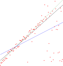
Comparison of the Theil–Sen estimator (black) and simple linear regression (blue) for a set of points with outliers. Because of the many outliers, neither of the regression lines fits the data well, as measured by the fact that neither gives a very high R2.
In statistics, the coefficient of determination, denoted R2 or r2 and pronounced «R squared», is the proportion of the variation in the dependent variable that is predictable from the independent variable(s).
It is a statistic used in the context of statistical models whose main purpose is either the prediction of future outcomes or the testing of hypotheses, on the basis of other related information. It provides a measure of how well observed outcomes are replicated by the model, based on the proportion of total variation of outcomes explained by the model.[1][2][3]
There are several definitions of R2 that are only sometimes equivalent. One class of such cases includes that of simple linear regression where r2 is used instead of R2. When only an intercept is included, then r2 is simply the square of the sample correlation coefficient (i.e., r) between the observed outcomes and the observed predictor values.[4] If additional regressors are included, R2 is the square of the coefficient of multiple correlation. In both such cases, the coefficient of determination normally ranges from 0 to 1.
There are cases where R2 can yield negative values. This can arise when the predictions that are being compared to the corresponding outcomes have not been derived from a model-fitting procedure using those data. Even if a model-fitting procedure has been used, R2 may still be negative, for example when linear regression is conducted without including an intercept,[5] or when a non-linear function is used to fit the data.[6] In cases where negative values arise, the mean of the data provides a better fit to the outcomes than do the fitted function values, according to this particular criterion.
The coefficient of determination can be more (intuitively) informative than MAE, MAPE, MSE, and RMSE in regression analysis evaluation, as the former can be expressed as a percentage, whereas the latter measures have arbitrary ranges. It also proved more robust for poor fits compared to SMAPE on the test datasets in the article.[7]
When evaluating the goodness-of-fit of simulated (Ypred) vs. measured (Yobs) values, it is not appropriate to base this on the R2 of the linear regression (i.e., Yobs= m·Ypred + b).[citation needed] The R2 quantifies the degree of any linear correlation between Yobs and Ypred, while for the goodness-of-fit evaluation only one specific linear correlation should be taken into consideration: Yobs = 1·Ypred + 0 (i.e., the 1:1 line).[8][9]
Definitions[edit]
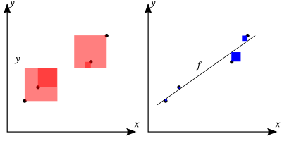

The better the linear regression (on the right) fits the data in comparison to the simple average (on the left graph), the closer the value of  is to 1. The areas of the blue squares represent the squared residuals with respect to the linear regression. The areas of the red squares represent the squared residuals with respect to the average value.
A data set has n values marked y1,…,yn (collectively known as yi or as a vector y = [y1,…,yn]T), each associated with a fitted (or modeled, or predicted) value f1,…,fn (known as fi, or sometimes ŷi, as a vector f).
Define the residuals as ei = yi − fi (forming a vector e).
If  is the mean of the observed data:

then the variability of the data set can be measured with two sums of squares formulas:
- The sum of squares of residuals, also called the residual sum of squares:

- The total sum of squares (proportional to the variance of the data):


The most general definition of the coefficient of determination is

In the best case, the modeled values exactly match the observed values, which results in  and
and  . A baseline model, which always predicts , will have
  . Models that have worse predictions than this baseline will have a negative .
Relation to unexplained variance[edit]
In a general form, R2 can be seen to be related to the fraction of variance unexplained (FVU), since the second term compares the unexplained variance (variance of the model’s errors) with the total variance (of the data):

As explained variance[edit]
Suppose R2 = 0.49. This implies that 49% of the variability of the dependent variable in the data set has been accounted for, and the remaining 51% of the variability is still unaccounted for.
For regression models, the regression sum of squares, also called the explained sum of squares, is defined as

In some cases, as in simple linear regression, the total sum of squares equals the sum of the two other sums of squares defined above:

See Partitioning in the general OLS model for a derivation of this result for one case where the relation holds. When this relation does hold, the above definition of R2 is equivalent to

where n is the number of observations (cases) on the variables.
In this form R2 is expressed as the ratio of the explained variance (variance of the model’s predictions, which is SSreg / n) to the total variance (sample variance of the dependent variable, which is SStot / n).
This partition of the sum of squares holds for instance when the model values ƒi have been obtained by linear regression. A milder sufficient condition reads as follows: The model has the form

where the qi are arbitrary values that may or may not depend on i or on other free parameters (the common choice qi = xi is just one special case), and the coefficient estimates  and
and  are obtained by minimizing the residual sum of squares.
This set of conditions is an important one and it has a number of implications for the properties of the fitted residuals and the modelled values. In particular, under these conditions:

As squared correlation coefficient[edit]
In linear least squares multiple regression with an estimated intercept term, R2 equals the square of the Pearson correlation coefficient between the observed  and modeled (predicted)
  data values of the dependent variable.
In a linear least squares regression with an intercept term and a single explanator, this is also equal to the squared Pearson correlation coefficient of the dependent variable and explanatory variable 
It should not be confused with the correlation coefficient between two explanatory variables, defined as

where the covariance between two coefficient estimates, as well as their standard deviations, are obtained from the covariance matrix of the coefficient estimates,  .
.
Under more general modeling conditions, where the predicted values might be generated from a model different from linear least squares regression, an R2 value can be calculated as the square of the correlation coefficient between the original and modeled data values. In this case, the value is not directly a measure of how good the modeled values are, but rather a measure of how good a predictor might be constructed from the modeled values (by creating a revised predictor of the form α + βƒi).[citation needed] According to Everitt,[10] this usage is specifically the definition of the term «coefficient of determination»: the square of the correlation between two (general) variables.
Interpretation[edit]
R2 is a measure of the goodness of fit of a model.[11] In regression, the R2 coefficient of determination is a statistical measure of how well the regression predictions approximate the real data points. An R2 of 1 indicates that the regression predictions perfectly fit the data.
Values of R2 outside the range 0 to 1 occur when the model fits the data worse than the worst possible least-squares predictor (equivalent to a horizontal hyperplane at a height equal to the mean of the observed data). This occurs when a wrong model was chosen, or nonsensical constraints were applied by mistake. If equation 1 of Kvålseth[12] is used (this is the equation used most often), R2 can be less than zero. If equation 2 of Kvålseth is used, R2 can be greater than one.
In all instances where R2 is used, the predictors are calculated by ordinary least-squares regression: that is, by minimizing SSres. In this case, R2 increases as the number of variables in the model is increased (R2 is monotone increasing with the number of variables included—it will never decrease). This illustrates a drawback to one possible use of R2, where one might keep adding variables (kitchen sink regression) to increase the R2 value. For example, if one is trying to predict the sales of a model of car from the car’s gas mileage, price, and engine power, one can include such irrelevant factors as the first letter of the model’s name or the height of the lead engineer designing the car because the R2 will never decrease as variables are added and will likely experience an increase due to chance alone.
This leads to the alternative approach of looking at the adjusted R2. The explanation of this statistic is almost the same as R2 but it penalizes the statistic as extra variables are included in the model. For cases other than fitting by ordinary least squares, the R2 statistic can be calculated as above and may still be a useful measure. If fitting is by weighted least squares or generalized least squares, alternative versions of R2 can be calculated appropriate to those statistical frameworks, while the «raw» R2 may still be useful if it is more easily interpreted. Values for R2 can be calculated for any type of predictive model, which need not have a statistical basis.
In a multiple linear model[edit]
Consider a linear model with more than a single explanatory variable, of the form

where, for the ith case,  is the response variable,
  are p regressors, and
  is a mean zero error term. The quantities
  are unknown coefficients, whose values are estimated by least squares. The coefficient of determination R2 is a measure of the global fit of the model. Specifically, R2 is an element of [0, 1] and represents the proportion of variability in Yi that may be attributed to some linear combination of the regressors (explanatory variables) in X.[13]
R2 is often interpreted as the proportion of response variation «explained» by the regressors in the model. Thus, R2 = 1 indicates that the fitted model explains all variability in , while R2 = 0 indicates no ‘linear’ relationship (for straight line regression, this means that the straight line model is a constant line (slope = 0, intercept = ) between the response variable and regressors). An interior value such as R2 = 0.7 may be interpreted as follows: «Seventy percent of the variance in the response variable can be explained by the explanatory variables. The remaining thirty percent can be attributed to unknown, lurking variables or inherent variability.»
A caution that applies to R2, as to other statistical descriptions of correlation and association is that «correlation does not imply causation.» In other words, while correlations may sometimes provide valuable clues in uncovering causal relationships among variables, a non-zero estimated correlation between two variables is not, on its own, evidence that changing the value of one variable would result in changes in the values of other variables. For example, the practice of carrying matches (or a lighter) is correlated with incidence of lung cancer, but carrying matches does not cause cancer (in the standard sense of «cause»).
In case of a single regressor, fitted by least squares, R2 is the square of the Pearson product-moment correlation coefficient relating the regressor and the response variable. More generally, R2 is the square of the correlation between the constructed predictor and the response variable. With more than one regressor, the R2 can be referred to as the coefficient of multiple determination.
Inflation of R2[edit]
In least squares regression using typical data, R2 is at least weakly increasing with increases in the number of regressors in the model. Because increases in the number of regressors increase the value of R2, R2 alone cannot be used as a meaningful comparison of models with very different numbers of independent variables. For a meaningful comparison between two models, an F-test can be performed on the residual sum of squares[citation needed], similar to the F-tests in Granger causality, though this is not always appropriate[further explanation needed]. As a reminder of this, some authors denote R2 by Rq2, where q is the number of columns in X (the number of explanators including the constant).
To demonstrate this property, first recall that the objective of least squares linear regression is

where Xi is a row vector of values of explanatory variables for case i and b is a column vector of coefficients of the respective elements of Xi.
The optimal value of the objective is weakly smaller as more explanatory variables are added and hence additional columns of  (the explanatory data matrix whose ith row is Xi) are added, by the fact that less constrained minimization leads to an optimal cost which is weakly smaller than more constrained minimization does. Given the previous conclusion and noting that
  depends only on y, the non-decreasing property of R2 follows directly from the definition above.
The intuitive reason that using an additional explanatory variable cannot lower the R2 is this: Minimizing  is equivalent to maximizing R2. When the extra variable is included, the data always have the option of giving it an estimated coefficient of zero, leaving the predicted values and the R2 unchanged. The only way that the optimization problem will give a non-zero coefficient is if doing so improves the R2.
Caveats[edit]
R2 does not indicate whether:
- the independent variables are a cause of the changes in the dependent variable;
- omitted-variable bias exists;
- the correct regression was used;
- the most appropriate set of independent variables has been chosen;
- there is collinearity present in the data on the explanatory variables;
- the model might be improved by using transformed versions of the existing set of independent variables;
- there are enough data points to make a solid conclusion.
Extensions[edit]
Adjusted R2[edit]
The use of an adjusted R2 (one common notation is  , pronounced «R bar squared»; another is
  or
or  ) is an attempt to account for the phenomenon of the R2 automatically increasing when extra explanatory variables are added to the model. There are many different ways of adjusting ([14]). By far the most used one, to the point that it is typically just referred to as adjusted R, is the correction proposed by Mordecai Ezekiel.[14][15]
The adjusted R2 is defined as

where dfres is the degrees of freedom of the estimate of the population variance around the model, and dftot is the degrees of freedom of the estimate of the population variance around the mean. dfres is given in terms of the sample size n and the number of variables p in the model, dfres =n − p. dftot is given in the same way, but with p being unity for the mean, i.e. dftot = n − 1.
Inserting the degrees of freedom and using the definition of R2, it can be rewritten as:

where p is the total number of explanatory variables in the model, and n is the sample size.
The adjusted R2 can be negative, and its value will always be less than or equal to that of R2. Unlike R2, the adjusted R2 increases only when the increase in R2 (due to the inclusion of a new explanatory variable) is more than one would expect to see by chance. If a set of explanatory variables with a predetermined hierarchy of importance are introduced into a regression one at a time, with the adjusted R2 computed each time, the level at which adjusted R2 reaches a maximum, and decreases afterward, would be the regression with the ideal combination of having the best fit without excess/unnecessary terms.
Adjusted R2 can be interpreted as a less biased estimator of the population R2, whereas the observed sample R2 is a positively biased estimate of the population value.[16] Adjusted R2 is more appropriate when evaluating model fit (the variance in the dependent variable accounted for by the independent variables) and in comparing alternative models in the feature selection stage of model building.[16]
The principle behind the adjusted R2 statistic can be seen by rewriting the ordinary R2 as

where  and
and  are the sample variances of the estimated residuals and the dependent variable respectively, which can be seen as biased estimates of the population variances of the errors and of the dependent variable. These estimates are replaced by statistically unbiased versions:
  and
and  .
.
Despite using unbiased estimators for the population variances of the error and the dependent variable, adjusted R2 is not an unbiased estimator of the population R2,[16] which results by using the population variances of the errors and the dependent variable instead of estimating them. Ingram Olkin and John W. Pratt derived the Minimum-variance unbiased estimator for the population R2,[17] which is known as Olkin-Pratt estimator. Comparisons of different approaches for adjusting R2 concluded that in most situations either an approximate version of the Olkin-Pratt estimator [16] or the exact Olkin-Pratt estimator [18] should be preferred over (Ezekiel) adjusted R2.
Coefficient of partial determination[edit]
The coefficient of partial determination can be defined as the proportion of variation that cannot be explained in a reduced model, but can be explained by the predictors specified in a full(er) model.[19][20][21] This coefficient is used to provide insight into whether or not one or more additional predictors may be useful in a more fully specified regression model.
The calculation for the partial R2 is relatively straightforward after estimating two models and generating the ANOVA tables for them. The calculation for the partial R2 is

which is analogous to the usual coefficient of determination:

Generalizing and decomposing R2[edit]
As explained above, model selection heuristics such as the Adjusted criterion and the F-test examine whether the total sufficiently increases to determine if a new regressor should be added to the model. If a regressor is added to the model that is highly correlated with other regressors which have already been included, then the total will hardly increase, even if the new regressor is of relevance. As a result, the above-mentioned heuristics will ignore relevant regressors when cross-correlations are high.[22]

Geometric representation of  .
.
Alternatively, one can decompose a generalized version of to quantify the relevance of deviating from a hypothesis.[22] As Hoornweg (2018) shows, several shrinkage estimators – such as Bayesian linear regression, ridge regression, and the (adaptive) lasso – make use of this decomposition of when they gradually shrink parameters from the unrestricted OLS solutions towards the hypothesized values. Let us first define the linear regression model as

It is assumed that the matrix is standardized with Z-scores and that the column vector is centered to have a mean of zero. Let the column vector  refer to the hypothesized regression parameters and let the column vector
  denote the estimated parameters. We can then define

An of 75% means that the in-sample accuracy improves by 75% if the data-optimized solutions are used instead of the hypothesized values. In the special case that is a vector of zeros, we obtain the traditional again.
The individual effect on of deviating from a hypothesis can be computed with  (‘R-outer’). This
  times matrix is given by

where  . The diagonal elements of exactly add up to . If regressors are uncorrelated and is a vector of zeros, then the
  diagonal element of simply corresponds to the value between
  and . When regressors
  and are correlated,
  might increase at the cost of a decrease in
  . As a result, the diagonal elements of may be smaller than 0 and, in more exceptional cases, larger than 1. To deal with such uncertainties, several shrinkage estimators implicitly take a weighted average of the diagonal elements of to quantify the relevance of deviating from a hypothesized value.[22] Click on the lasso for an example.
R2 in logistic regression[edit]
In the case of logistic regression, usually fit by maximum likelihood, there are several choices of pseudo-R2.
One is the generalized R2 originally proposed by Cox & Snell,[23] and independently by Magee:[24]

where  is the likelihood of the model with only the intercept,
  is the likelihood of the estimated model (i.e., the model with a given set of parameter estimates) and n is the sample size. It is easily rewritten to:

where D is the test statistic of the likelihood ratio test.
Nico Nagelkerke noted that it had the following properties:[25][26]
- It is consistent with the classical coefficient of determination when both can be computed;
- Its value is maximised by the maximum likelihood estimation of a model;
- It is asymptotically independent of the sample size;
- The interpretation is the proportion of the variation explained by the model;
- The values are between 0 and 1, with 0 denoting that model does not explain any variation and 1 denoting that it perfectly explains the observed variation;
- It does not have any unit.
However, in the case of a logistic model, where  cannot be greater than 1, R2 is between 0 and
  : thus, Nagelkerke suggested the possibility to define a scaled R2 as R2/R2max.[27]
Comparison with norm of residuals[edit]
Occasionally, the norm of residuals is used for indicating goodness of fit. This term is calculated as the square-root of the sum of squares of residuals:

Both R2 and the norm of residuals have their relative merits. For least squares analysis R2 varies between 0 and 1, with larger numbers indicating better fits and 1 representing a perfect fit. The norm of residuals varies from 0 to infinity with smaller numbers indicating better fits and zero indicating a perfect fit. One advantage and disadvantage of R2 is the  term acts to normalize the value. If the yi values are all multiplied by a constant, the norm of residuals will also change by that constant but R2 will stay the same. As a basic example, for the linear least squares fit to the set of data:
| x | 1 | 2 | 3 | 4 | 5 |
|---|---|---|---|---|---|
| y | 1.9 | 3.7 | 5.8 | 8.0 | 9.6 |
R2 = 0.998, and norm of residuals = 0.302.
If all values of y are multiplied by 1000 (for example, in an SI prefix change), then R2 remains the same, but norm of residuals = 302.
Another single-parameter indicator of fit is the RMSE of the residuals, or standard deviation of the residuals. This would have a value of 0.135 for the above example given that the fit was linear with an unforced intercept.[28]
History[edit]
The creation of the coefficient of determination has been attributed to the geneticist Sewall Wright and was first published in 1921.[29]
See also[edit]
- Anscombe’s quartet
- Fraction of variance unexplained
- Goodness of fit
- Nash–Sutcliffe model efficiency coefficient (hydrological applications)
- Pearson product-moment correlation coefficient
- Proportional reduction in loss
- Regression model validation
- Root mean square deviation
- Stepwise regression
Notes[edit]
- ^ Steel, R. G. D.; Torrie, J. H. (1960). Principles and Procedures of Statistics with Special Reference to the Biological Sciences. McGraw Hill.
- ^ Glantz, Stanton A.; Slinker, B. K. (1990). Primer of Applied Regression and Analysis of Variance. McGraw-Hill. ISBN 978-0-07-023407-9.
- ^ Draper, N. R.; Smith, H. (1998). Applied Regression Analysis. Wiley-Interscience. ISBN 978-0-471-17082-2.
- ^ Devore, Jay L. (2011). Probability and Statistics for Engineering and the Sciences (8th ed.). Boston, MA: Cengage Learning. pp. 508–510. ISBN 978-0-538-73352-6.
- ^ Barten, Anton P. (1987). «The Coeffecient of Determination for Regression without a Constant Term». In Heijmans, Risto; Neudecker, Heinz (eds.). The Practice of Econometrics. Dordrecht: Kluwer. pp. 181–189. ISBN 90-247-3502-5.
- ^ Colin Cameron, A.; Windmeijer, Frank A.G. (1997). «An R-squared measure of goodness of fit for some common nonlinear regression models». Journal of Econometrics. 77 (2): 1790–2. doi:10.1016/S0304-4076(96)01818-0.
- ^ Chicco, Davide; Warrens, Matthijs J.; Jurman, Giuseppe (2021). «The coefficient of determination R-squared is more informative than SMAPE, MAE, MAPE, MSE and RMSE in regression analysis evaluation». PeerJ Computer Science. 7 (e623): e623. doi:10.7717/peerj-cs.623. PMC 8279135. PMID 34307865.
- ^ Legates, D.R.; McCabe, G.J. (1999). «Evaluating the use of «goodness-of-fit» measures in hydrologic and hydroclimatic model validation». Water Resour. Res. 35 (1): 233–241. Bibcode:1999WRR….35..233L. doi:10.1029/1998WR900018.
- ^ Ritter, A.; Muñoz-Carpena, R. (2013). «Performance evaluation of hydrological models: statistical significance for reducing subjectivity in goodness-of-fit assessments». Journal of Hydrology. 480 (1): 33–45. Bibcode:2013JHyd..480…33R. doi:10.1016/j.jhydrol.2012.12.004.
- ^ Everitt, B. S. (2002). Cambridge Dictionary of Statistics (2nd ed.). CUP. p. 78. ISBN 978-0-521-81099-9.
- ^ Casella, Georges (2002). Statistical inference (Second ed.). Pacific Grove, Calif.: Duxbury/Thomson Learning. p. 556. ISBN 9788131503942.
- ^ Kvalseth, Tarald O. (1985). «Cautionary Note about R2». The American Statistician. 39 (4): 279–285. doi:10.2307/2683704. JSTOR 2683704.
- ^ «Linear Regression — MATLAB & Simulink». www.mathworks.com.
- ^ a b Raju, Nambury S.; Bilgic, Reyhan; Edwards, Jack E.; Fleer, Paul F. (1997). «Methodology review: Estimation of population validity and cross-validity, and the use of equal weights in prediction». Applied Psychological Measurement. 21 (4): 291–305. doi:10.1177/01466216970214001. ISSN 0146-6216. S2CID 122308344.
- ^ Yin, Ping; Fan, Xitao (January 2001). «Estimating R 2 Shrinkage in Multiple Regression: A Comparison of Different Analytical Methods». The Journal of Experimental Education. 69 (2): 203–224. doi:10.1080/00220970109600656. ISSN 0022-0973. S2CID 121614674. Retrieved 2021-04-23.
- ^ a b c d Shieh, Gwowen (2008-04-01). «Improved shrinkage estimation of squared multiple correlation coefficient and squared cross-validity coefficient». Organizational Research Methods. 11 (2): 387–407. doi:10.1177/1094428106292901. ISSN 1094-4281. S2CID 55098407.
- ^ Olkin, Ingram; Pratt, John W. (March 1958). «Unbiased estimation of certain correlation coefficients». The Annals of Mathematical Statistics. 29 (1): 201–211. doi:10.1214/aoms/1177706717. ISSN 0003-4851.
- ^ Karch, Julian (2020-09-29). «Improving on Adjusted R-Squared». Collabra: Psychology. 6 (45). doi:10.1525/collabra.343. ISSN 2474-7394.
- ^ Richard Anderson-Sprecher, «Model Comparisons and R2«, The American Statistician, Volume 48, Issue 2, 1994, pp. 113–117.
- ^ (generalized to Maximum Likelihood) N. J. D. Nagelkerke, «A Note on a General Definition of the Coefficient of Determination», Biometrika, Vol. 78, No. 3. (Sep., 1991), pp. 691–692.
- ^ «regression — R implementation of coefficient of partial determination». Cross Validated.
- ^ a b c Hoornweg, Victor (2018). «Part II: On Keeping Parameters Fixed». Science: Under Submission. Hoornweg Press. ISBN 978-90-829188-0-9.
- ^ Cox, D. D.; Snell, E. J. (1989). The Analysis of Binary Data (2nd ed.). Chapman and Hall.
- ^ Magee, L. (1990). «R2 measures based on Wald and likelihood ratio joint significance tests». The American Statistician. 44 (3): 250–3. doi:10.1080/00031305.1990.10475731.
- ^ Nagelkerke, Nico J. D. (1992). Maximum Likelihood Estimation of Functional Relationships, Pays-Bas. Lecture Notes in Statistics. Vol. 69. ISBN 978-0-387-97721-8.
- ^ NJD Nagelkerke (September 1991). «A note on a general definition of the coefficient of determination». Biometrika. 78 (3): 691–692. doi:10.1093/biomet/78.3.691.
- ^ Nagelkerke, N. J. D. (1991). «A Note on a General Definition of the Coefficient of Determination». Biometrika. 78 (3): 691–2. doi:10.1093/biomet/78.3.691. JSTOR 2337038.
- ^ OriginLab webpage, http://www.originlab.com/doc/Origin-Help/LR-Algorithm. Retrieved February 9, 2016.
- ^ Wright, Sewall (January 1921). «Correlation and causation». Journal of Agricultural Research. 20: 557–585.
Further reading[edit]
- Gujarati, Damodar N.; Porter, Dawn C. (2009). Basic Econometrics (Fifth ed.). New York: McGraw-Hill/Irwin. pp. 73–78. ISBN 978-0-07-337577-9.
- Hughes, Ann; Grawoig, Dennis (1971). Statistics: A Foundation for Analysis. Reading: Addison-Wesley. pp. 344–348. ISBN 0-201-03021-7.
- Kmenta, Jan (1986). Elements of Econometrics (Second ed.). New York: Macmillan. pp. 240–243. ISBN 978-0-02-365070-3.
- Lewis-Beck, Michael S.; Skalaban, Andrew (1990). «The R-Squared: Some Straight Talk». Political Analysis. 2: 153–171. doi:10.1093/pan/2.1.153. JSTOR 23317769.
- Chicco, Davide; Warrens, Matthijs J.; Jurman, Giuseppe (2021). «The coefficient of determination R-squared is more informative than SMAPE, MAE, MAPE, MSE and RMSE in regression analysis evaluation». PeerJ Computer Science. 7 (e623): e623. doi:10.7717/peerj-cs.623. PMC 8279135. PMID 34307865.
R-квадрат (R2 или Коэффициент детерминации) — это статистическая мера, которая показывает степень вариации зависимой переменной из-за независимой переменной. В инвестировании он действует как полезный инструмент для технического анализа. Он оценивает эффективность ценной бумаги или фонда (зависимая переменная) по отношению к заданному эталонному индексу (независимая переменная).

В отличие от корреляции (R), которая измеряет силу связи между двумя переменными, R-квадрат указывает на изменение данных, объясняемое связью между независимой переменной. Независимая переменная. Независимая переменная — это объект, период времени или входное значение, изменения которого используется для оценки влияния на выходное значение (т. е. конечную цель), которое измеряется в математическом, статистическом или финансовом моделировании. Подробнее и зависимая переменная. Значение R2 находится в диапазоне от 0 до 1 и выражается в процентах. В финансах он указывает процент, на который ценные бумаги перемещаются в ответ на движение индекса. Чем выше значение R-квадрата, тем синхроннее движение ценных бумаг с индексом и наоборот. В результате это помогает инвесторам отслеживать свои инвестиции.
Оглавление
- Значение R-квадрата
- Формула R-квадрата
- Примеры расчета
- Пример №1
- Пример #2
- Интерпретация R-квадрата
- R-квадрат против скорректированного R-квадрата
- R против R-квадрат
- Часто задаваемые вопросы (FAQ)
- Рекомендуемые статьи
- R-квадрат измеряет степень движения зависимой переменной (акции или фонды) по отношению к независимой переменной (эталонный индекс).
- Это помогает узнать производительность ценной бумаги по эталонному индексу.
- Чем выше значение R2, тем больше зависимость зависимой переменной от независимой переменной и наоборот.
- Значения R2 представлены в процентах в диапазоне от 1 до 100 процентов.
- R, R2 и скорректированный R2 — это разные термины в статистике. R представляет собой корреляцию между переменными, R2 указывает на изменение данных, объясняемое корреляцией, а скорректированный R2 учитывает другие переменные.
Формула R-квадрата
Чтобы добраться до R2, сделайте следующее:
1. Определите коэффициент корреляцииКоэффициент корреляцииКоэффициент корреляции, иногда называемый коэффициентом взаимной корреляции, представляет собой статистическую меру, используемую для оценки силы взаимосвязи между двумя переменными. Его значения варьируются от -1,0 (отрицательная корреляция) до +1,0 (положительная корреляция). читать дальше (р)

где,
- n = количество наблюдений
- Σx = общее значение независимой переменной
- Σy = общее значение зависимой переменной
- Σxy = сумма произведения независимой и зависимой переменных
- Σx2 = сумма квадратов значения независимой переменной
- Σy2 = сумма квадратов значения зависимой переменной
2. Возведите в квадрат коэффициент корреляции (R)

Значение R2 лежит в диапазоне от 0 до 1. Это означает, что если значение равно 0, независимая переменная не объясняет изменения зависимой переменной. Однако значение 1 показывает, что независимая переменная прекрасно объясняет изменение зависимой переменной. Обычно R2 выражается в процентах для удобства.
Примеры расчета
Вот несколько примеров, чтобы прояснить концепцию R-квадрата.
Пример №1
Выясним зависимость между количеством статей, написанных журналистами в месяц, и их многолетним стажем. Здесь зависимая переменная (y) — количество написанных статей, а независимая переменная (x) — количество лет опыта.
Сначала найдите коэффициент корреляции (R), а затем возведите его в квадрат, чтобы получить коэффициент детерминацииКоэффициент детерминацииКоэффициент детерминации, также известный как R в квадрате, определяет степень дисперсии зависимой переменной, которую можно объяснить независимой переменной. Следовательно, чем выше коэффициент, тем лучше уравнение регрессии, так как это означает, что независимая переменная выбрана с умом. Подробнее или R2. Вот данные.


R2 = 0,932 = 0,8649
Следовательно, коэффициент детерминации составляет 86%. Это означает, что 86% различий в количестве написанных статей объясняются многолетним опытом автора.
Пример #2
Предположим, инвестор хочет контролировать свой портфель, просматривая индекс S&P. Поэтому он хочет знать корреляцию между доходностью своего портфеля. Доходность портфеля. Формула доходности портфеля вычисляет доходность всего портфеля, состоящего из различных отдельных активов. Формула рассчитывается путем вычисления рентабельности инвестиций в отдельный актив, умноженной на соответствующую весовую категорию в общем портфеле, и сложения всех результатов вместе. Rp = ∑ni=1 wi riчитать далее и эталонный индекс. Итак, он вычисляет R и R-квадрат. Высокое значение R-квадрата указывает на то, что портфель движется подобно индексу.
Вот список доходности портфеля, представленной зависимой переменной (y), и доходности эталонного индекса, обозначенной независимой переменной (x).

Наконец, R2 рассчитывается по формуле:


Р2 = [0.8759 ]2
= 0,7672
Значение R2 подразумевает, что вариация доходности портфеля на 76,72% соответствует индексу S&P. Таким образом, инвестор может отслеживать движения своего портфеля, следя за индексом.
Интерпретация R-квадрата
R-квадрат измеряет влияние изменения независимой переменной на изменение зависимой переменной. На фондовых рынках это процент, на который ценные бумаги изменяются в ответ на движение эталонного индекса, такого как индекс S&P.
Если кто-то хочет, чтобы портфель ценных бумаг синхронизировался с эталонным индексом, он должен иметь высокое значение R2. Однако, если кто-то хочет, чтобы эталонный тест не влиял на производительность портфеля ценных бумаг, ему нужно искать портфель с низким значением R2.
Другими словами, если значение R2 находится в диапазоне:
- 70-100 %, тогда портфель ценных бумаг имеет наибольшую связь с движением и доходностью эталонных индексов.
- 40-70%, то соотношение между доходностью портфеля и доходностью эталонных индексов среднее
- 1-40%, то связь между доходностью портфеля и доходностью эталонного индекса очень мала или отсутствует.
R-квадрат против скорректированного R-квадрата
И R2, и скорректированный R2 используются для измерения корреляции между зависимой переменной и независимой переменной. С одной стороны, R2 представляет собой процент дисперсии зависимой переменной, описываемой независимой переменной. С другой стороны, скорректированный R2 представляет собой пересмотренную версию R-квадрата, скорректированную с учетом количества используемых независимых переменных.
Скорректированный R-квадрат Скорректированный R-квадрат Скорректированный R-квадрат относится к статистическому инструменту, который помогает инвесторам измерять степень дисперсии зависимой переменной, которая может быть объяснена независимой переменной, и учитывает влияние только тех независимых переменных, которые оказывают влияние на изменение зависимой переменной. Читать далее обеспечивает более точную корреляцию между переменными, учитывая влияние всех независимых переменных на функцию регрессии. В результате легко определить точные переменные, влияющие на корреляцию. Кроме того, это помогает узнать, какие переменные более важны, чем другие.
R-квадрат имеет тенденцию к увеличению при добавлении независимых переменных в набор данных. Однако скорректированный R2 может устранить этот недостаток. Следовательно, всякий раз, когда добавленные переменные несущественны или отрицательны, скорректированное значение R2 соответственно уменьшается или корректируется. Следовательно, можно сказать, что скорректированный R2 более надежен, чем R2.
R против R-квадрат
R или коэффициент корреляции — это термин, который передает прямую связь между любыми двумя переменными, такими как доходность и риск ценной бумаги. Диапазон R составляет от -1 до 1. Отрицательное значение указывает на обратную связь, а +1 указывает на прямую связь между переменными.
R2 используется в наборе данных, который содержит несколько переменных с различными свойствами, такими как риск, доходность, процентная ставка и срок погашения ценных бумаг. Диапазон R2 составляет от 0 до 1, где 0 — плохой показатель, а 1 — отличный.
Часто задаваемые вопросы (FAQ)
Что означает R-квадрат?
В функции регрессии R2 означает меру взаимосвязи между зависимой и независимой переменными. Его также называют коэффициентом детерминации в статистике. В финансовой терминологии R2 представляет отношение безопасности портфеля к эталонному индексу. Более высокое значение R2 означает, что эталонный индекс представляет производительность портфеля ценных бумаг и наоборот.
Что такое идеальное значение R-квадрата?
Значение R2 находится в диапазоне от 0 до 1 и выражается в процентах. Более высокий процент, близкий к 100%, указывает на то, что независимая переменная, выбранная для определения зависимой переменной, является идеальной, и наоборот. При инвестировании желательным считается значение R2 70% и более.
Как рассчитывается R-квадрат?
R2 можно рассчитать по следующей формуле:
где n — количество наблюдений, x — независимая переменная, а y — зависимая переменная.
Рекомендуемые статьи
Эта статья была руководством по R-Squared и его значению. Здесь мы обсуждаем формулу R-Squared, интерпретацию значений в регрессии, примеры и различия с R. Вы можете узнать больше об экономике из следующих статей:
- Эконометрика
- Формула множественной регрессии
- Нелинейная регрессия
коэффициент детерминации ( — R-квадрат) — это доля дисперсии зависимой переменной, объясняемая рассматриваемой моделью зависимости, то есть объясняющими переменными. Более точно — это единица минус доля необъясненной дисперсии (дисперсии случайной ошибки модели, или условной по факторам дисперсии зависимой переменной) в дисперсии зависимой переменной. Его рассматривают как универсальную меру зависимости одной случайной величины от множества других. В частном случае линейной зависимости является квадратом так называемого множественного коэффициента корреляции между зависимой переменной и объясняющими переменными. В частности, для модели парной линейной регрессии коэффициент детерминации равен квадрату обычного коэффициента корреляции между y и x.
Содержание
- 1 Определение и формула
- 1.1 Интерпретация
- 2 Недостаток и альтернативные показатели
- 2.1 Скорректированный (adjusted)
- 2.2 Информационные критерии
- 2.3 -обобщенный (extended)
- 3 Замечание
- 4 Вау!! 😲 Ты еще не читал? Это зря!
- 5 Примечания
- 6 Ссылки
Определение и формула[править ]
Истинный коэффициент детерминации модели зависимости случайной величины y от факторов x определяется следующим образом:

где  — условная (по факторам x) дисперсия зависимой переменной (дисперсия случайной ошибки модели).
В данном определении используются истинные параметры, характеризующие распределение случайных величин. Если использовать выборочную оценку значений соответствующих дисперсий, то получим формулу для выборочного коэффициента детерминации (который обычно и подразумевается под коэффициентом детерминации):

где  — сумма квадратов остатков регрессии,
  — фактические и расчетные значения объясняемой переменной.
 — общая сумма квадратов.

В случае линейной регрессии с константой  , где
, где 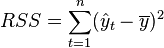 — объясненная сумма квадратов, поэтому получаем более простое определение в этом случае — коэффициент детерминации — это доля объясненной суммы квадратов в общей:

Необходимо подчеркнуть, что эта формула справедлива только для модели с константой, в общем случае необходимо использовать предыдущую формулу.
Интерпретация[править ]
- Коэффициент детерминации для модели с константой принимает значения от 0 до 1 . Об этом говорит сайт https://intellect.icu . Чем ближе значение коэффициента к 1, тем сильнее зависимость. При оценке регрессионных моделей это интерпретируется как соответствие модели данным. Для приемлемых моделей предполагается, что коэффициент детерминации должен быть хотя бы не меньше 50 % (в этом случае коэффициент множественной корреляции превышает по модулю 70 %). Модели с коэффициентом детерминации выше 80 % можно признать достаточно хорошими (коэффициент корреляции превышает 90 %). Значение коэффициента детерминации 1 означает функциональную зависимость между переменными.
- При отсутствии статистической связи между объясняемой переменной и факторами, статистика для линейной регрессии имеет асимптотическое распределение , где — количество факторов модели (см. тест множителей Лагранжа). В случае линейной регрессии с нормально распределенными случайными ошибками статистика имеет точное (для выборок любого объема) распределение Фишера (см. F- тест ). Информация о распределении этих величин позволяет проверить статистическую значимость регрессионной модели исходя из значения коэффициента детерминации. Фактически в этих тестах проверяется гипотеза о равенстве истинного коэффициента детерминации нулю.
- В общем случае коэффициент детерминации может быть и отрицательным, это говорит о крайней неадекватности модели: простое среднее приближает лучше.
 для линейной регрессии имеет асимптотическое распределение
  , где
, где  — количество факторов модели (см. тест множителей Лагранжа). В случае линейной регрессии с нормально распределенными случайными ошибками статистика
 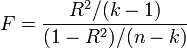 имеет точное (для выборок любого объема) распределение Фишера
 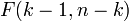 (см. F- тест ). Информация о распределении этих величин позволяет проверить статистическую значимость регрессионной модели исходя из значения коэффициента детерминации. Фактически в этих тестах проверяется гипотеза о равенстве истинного коэффициента детерминации нулю.
Недостаток и альтернативные показатели[править ]
Основная проблема применения (выборочного) заключается в том, что его значение увеличивается (не уменьшается) от добавления в модель новых переменных, даже если эти переменные никакого отношения к объясняемой переменной не имеют! Поэтому сравнение моделей с разным количеством факторов с помощью коэффициента детерминации, вообще говоря, некорректно. Для этих целей можно использовать альтернативные показатели.
Скорректированный (adjusted) [править ]
Для того, чтобы была возможность сравнивать модели с разным числом факторов так, чтобы число регрессоров (факторов) не влияло на статистику обычно используется скорректированный коэффициент детерминации, в котором используются несмещенные оценки дисперсий:

который дает штраф за дополнительно включенные факторы, где n — количество наблюдений, а k — количество параметров.
Данный показатель всегда меньше единицы, но теоретически может быть и меньше нуля (только при очень маленьком значении обычного коэффициента детерминации и большом количестве факторов). Поэтому теряется интерпретация показателя как «доли». Тем не менее, применение показателя в сравнении вполне обоснованно.
Для моделей с одинаковой зависимой переменной и одинаковым объемом выборки сравнение моделей с помощью скорректированного коэффициента детерминации эквивалентно их сравнению с помощью остаточной дисперсии 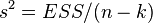 или стандартной ошибки модели
  . Разница только в том, что последние критерии чем меньше, тем лучше.
Информационные критерии[править ]
AIC — информационный критерий Акаике — применяется исключительно для сравнения моделей. Чем меньше значение, тем лучше. Часто используется для сравнения моделей временных рядов с разным количеством лагов.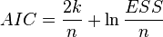 , где k— количество параметров модели.
BIC или SC — байесовский информационный критерий Шварца — используется и интерпретируется аналогично AIC.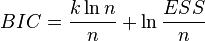 . Дает больший штраф за включение лишних лагов в модель , чем AIC.
-обобщенный (extended)[править ]
В случае отсутствия в линейной множественной МНК регрессии константы свойства коэффициента детерминации могут нарушаться для конкретной реализации. Поэтому модели регрессии со свободным членом и без него нельзя сравнивать по критерию . Эта проблема решается с помощью построения обобщенного коэффициента детерминации  , который совпадает с исходным для случая МНК регрессии со свободным членом, и для которого выполняются четыре свойства, перечисленные выше. Суть этого метода заключается в рассмотрении проекции единичного вектора на плоскость объясняющих переменных.
Для случая регрессии без свободного члена: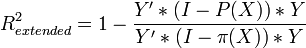 ,
,
где X — матрица nxk значений факторов,  — проектор на плоскость X,
 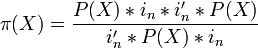 , где
, где  — единичный вектор nx1.
с условием небольшой модификации, также подходит для сравнения между собой регрессий, построенных с помощью: МНК, обобщенного метода наименьших квадратов (ОМНК), условного метода наименьших квадратов (УМНК), обобщенно-условного метода наименьших квадратов (ОУМНК).
Замечание[править ]
Высокие значения коэффициента детерминации, вообще говоря, не свидетельствуют о наличии причинно-следственной зависимости между переменными (также как и в случае обычного коэффициента корреляции). Например, если объясняемая переменная и факторы, на самом деле не связанные с объясняемой переменой, имеют возрастающую динамику, то коэффициент детерминации будет достаточно высок. Поэтому логическая и смысловая адекватность модели имеют первостепенную важность. Кроме того, необходимо использовать критерии для всестороннего анализа качества модели .
Вау!! 😲 Ты еще не читал? Это зря![править ]
- Коэффициент корреляции
- Корреляция
- Мультиколлинеарность
- Дисперсия случайной величины
- Метод группового учета аргументов
- Регрессионный анализ
Примечания[править ]
Напиши свое отношение про коэффициент детерминации. Это меня вдохновит писать для тебя всё больше и больше интересного. Спасибо Надеюсь, что теперь ты понял что такое коэффициент детерминации
и для чего все это нужно, а если не понял, или есть замечания,
то нестесняся пиши или спрашивай в комментариях, с удовольствием отвечу. Для того чтобы глубже понять настоятельно рекомендую изучить всю информацию из категории
Теория вероятностей. Математическая статистика и Стохастический анализ