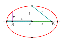
Эллипсом называют плоскую кривую, состоящую из точек, сумма расстояний которых от двух определённых точек плоскости является неизменной, строго заданной величиной, равной суммарной длине двух больших его полуосей (2a). Эти две точки называются фокусами эллипса.
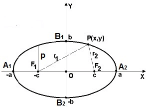
F1 и F2 – фокусы эллипса;
а – большая полуось;
b – малая полуось
с – фокусное расстояние
Теорема
Фокусное расстояние эллипса и его полуоси связаны между собой соотношением [boldsymbol{a^{2}=b^{2}+c^{2}}]
Доказательство:
Когда точка M на линии эллипса находится на его пересечении с вертикальной осью, из теоремы Пифагора выходит, что
r1 + r2 = 2*√(b2 + c2)
Когда точка M пересекает горизонтальную ось
r1 + r2 = а – c + а + c
По определению эллипса r1 + r 2 = const
Это позволяет после приравнивания получить
a² = b² + c²
r1 + r2 = 2а
Что и требовалось доказать.
Уравнение эллипса
Каноническим уравнением эллипса называют уравнение [boldsymbol{1=left(x^{2} / a^{2}right)+left(y^{2} / b^{2}right)}]
Доказательство уравнения:
Введём прямоугольную декартову систему координат.
Сначала докажем, что координаты любой из точек на эллипсе удовлетворяют приведённому каноническому уравнению. Затем покажем, что любое из решений уравнения является координатами точки, лежащей на линии эллипса. Из этого будет следовать удовлетворение каноническому уравнению только тех точек, которые лежат на поверхности эллипса. Опираясь на этот факт и на определение эллипса можно будет однозначно сделать вывод, что написанное нами уравнением является каноническим уравнением или, как ещё говорят, основной формулой эллипса.
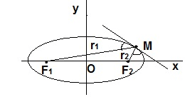
- Пусть М(х, у) будет точкой эллипса, т.е. сумму её фокальных радиусов примем равной 2а, т. е. r1 + r2 = 2a.
С помощью формулы расстояния, разделяющего две точки на координатной плоскости, можно легко найти фокальные радиусы точки M.r1 = √[(x + c)2 + y2]
r2 = √[(x — c)2 + y2]Из этих уравнений получаем √[(x + c)2 + y2] + √[(x — c)2 + y2] = 2a
Если один из корней перенести в правую часть и возвести всё в квадрат, то придём к выражению
(x + c)2 + y2 = 4a2 – 4a√[(x — c)2 + y2] + (x – c)2 + y2После сокращения приходим к 2xc = 4a2 – 4a√[(x-c)2 + y2] – 2xc
После приведения подобных членов, сокращения на 4 и уединения радикала будем иметь
a√[(x-c)2 + y2] = a2 – xcВозведём это выражение в квадрат
a2(x-c)2 + a2 y2 = a4 – 2a2xc + x2c2Если раскрыть скобки и сократить на -2a2 xc, то a2x2 + a2c2 + a2y2 = a4 + x2c2
Отсюда легко получить (a2 – c2)x2 + a2y2 = a2(a2 – c2)
Из этого следует, что b2x2 +a2y2 = a2b2 - Пусть некоторые числа (x, y) полностью удовлетворяют каноническому уравнению
1 = (x2/a2) + (y2/b2)
Пусть нам дана точка M(x,y) на координатной плоскости 0xy
Из канонического уравнения следует, что Y2 = b2(1- x2/a2)
Если это равенство подставить в выражение для фокальных радиусов, которые имеет точка M, то можно получить
r1 = √[(x + c)2 +y2] = √[x2 +2xc + c2 +b2 – b2x2/a2] = √[x2(1 – b2/a2) + 2xc +c2 +b2] =
= √[x2(a2 – b2)/a2 + 2xc + (c2 + b2)] = √[x2 (c2/a2) + 2xc +a2] = √[x(c/a) +a]2 = |a +xε|
т. е. r1 = |a +xε|
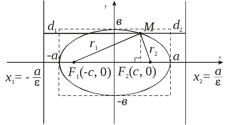
Отношение 2с/2a = c/a = ε называется эксцентриситетом эллипса. Оно у него всегда меньше 1.
То же самое просчитываем для r2.
Т. к. x2/a2 больше или равно 1 или x больше или равно большой полуоси (a), то можно сделать вывод о справедливости неравенства a≥|x|> |x|* ε = |xε|
Отсюда явно следует, что a+-|xε|>0 или a+-xε > 0 и r1 = a + xε, r2 = a — xε
Из полученных равенств выходит, что r1 + r2 = 2a, это значит, что точка M однозначно является точкой эллипса. Это нам и нужно было доказать.
Свойства эллипса
- У эллипса имеются две взаимно перпендикулярные оси симметрии.
Доказательство:
Переменные x и y в уравнение эллипса входят лишь во второй степени. Это означает, что если точка M с координатами (x,y) ему принадлежит, то и точки М1 (-x, y) и M2 (x, -y) тоже принадлежат ему. Легко проверить, что указанные координаты удовлетворяют каноническому уравнению эллипса. M1 симметрична по отношению к оси X, а M2 по отношению к оси Y. Получается, что у эллипса есть две взаимно перпендикулярные точки симметрии. - У эллипса есть центр симметрии.
Доказательство:
Если координаты точки М(x,y) будут удовлетворять уравнению эллипса, то и точка
N (–x; –y) ему тоже будет удовлетворять. M и N симметричны по отношению к началу координат. Это как раз и означает, что у эллипса имеется центр симметрии. - Эллипс пересекает каждую из осей в двух точках.
Доказательство:
Возьмём произвольную точку эллипса M(x,y). Расстояние этой точки до фокусов будетr1 = √[(x + c)2 + y2]
r2 = √[(x — c)2 + y2]Теперь давайте рассмотрим выражение
(x+-c)2 + y2 = x2 +- 2xc + c2+ y2 =
= x2 +- 2xc + a2 – b2 +y2 = x2 +- 2xc+ a2 — b2 + b2(1-x2/a2) =
= (a2 – b2)*x2/a2 +-2xc +a2 = c2*x2/a2+-2xa(c/a) + a2 = (a +c*x/a)2Эксцентриситет эллипса, как сказано ранее, меньше 1. Т. к. |x|≤ a, то a – εx > 0. Поэтому
F1M = a + εx и F2M = a – εx. Напомним, что ε – это эксцентриситет эллипса.
А теперь несколько свойств эллипса без доказательств.
- Эллипс можно получить, сжав окружность.
- Если через эллипс проходят две прямые, то отрезок, концами которого являются середины отрезков созданных при пересечении прямых, обязательно пересекает середину, центр эллипса.
- Угол, созданный касательной к эллипсу и его радиусом, проходящем через фокусы указанной геометрической фигуры, в любых случаях пересекает середину эллипса.
- Уравнение касательной к эллипсу в точке М, имеющей координаты xM и yM
1 = (x*xM)/a2 + (y*yM)/b2 - Эволюта эллипса представляет собой астероиду, растянутую вдоль его малой оси.
- Угол между касательной к эллипсу и одним его фокальным радиусом (r1) имеет ту же величину, что и угол, разделяющий касательную и другой фокальный радиус (r2) фигуры.
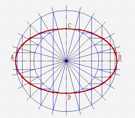
Как построить эллипс
Расскажем, как построить эллипс по его большой и малой полуосям и с помощью циркуля.
Построение эллипса по его большой и малой осям
Считается самым простым, не требующим серьёзных навыков.
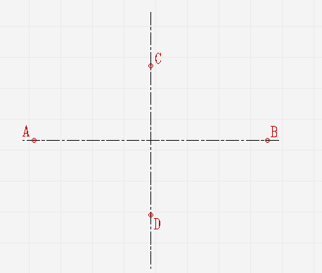
Проведите две перпендикулярные оси;
От места пересечения осей на вертикальной отложите верх и вниз отрезки. Они будут составлять малую ось эллипса. На горизонтальной отложите отрезки вправо и влево. Из них будет состоять большая ось;
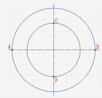
Проведите две концентрические окружности. Одну диаметром AB, диаметром CD;
Проведите ещё диаметры в различных направлениях;
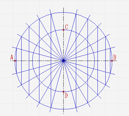
В местах, где лучи соприкасаются с окружностями, проведите линии параллельные малой и большой осям эллипса, пока они не пересекутся в точках, которые принадлежат эллипсу;
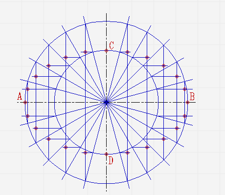
Соедините полученные точки плавной линией.

Нет времени решать самому?
Наши эксперты помогут!
Как построить эллипс с помощью циркуля
Во многом здесь всё аналогично предыдущему способу, поэтому перегружать текст иллюстрациями не будем.
Порядок действий следующий:
- Проведите две перпендикулярные линии. Они будут осями эллипса, а точка их пересечения центром геометрической фигуры;
- Определитесь с величиной большой и малой полуосей, если их значения не заданы в условии задачи;
- Установите раствор циркуля на длину большой полуоси (a). Поместите циркуль в точку O и отметьте на одной из линий две точки, P1 и P2. Установите раствор циркуля на длину малой полуоси. Опять поместите его в точку O и отметьте на другой из линий ещё две точки, обозначьте их как Q1 и Q2. Отрезки P1P2 и Q1Q2 будут большой и малой полуосями будущего эллипса;
- Установите раствор циркуля на величину a. Поместите циркуль в точке Q1 или Q2. После этого обозначьте циркулем на отрезке P1P2 точки F1 и F2. Это будут фокусы фигуры.
- Отметьте на P1P2 любую точку и обозначьте её T. Поставьте в этой точке циркуль и измерьте этим инструментом расстояние до P1. Затем начертите окружность данного радиуса из фокуса F1. После этого нужно сделать ещё одну окружность с радиусом величиной с расстояние от T до P2, но уже с центром из F2;
- Отметьте точки, в которых пересекаются обе окружности. Повторяйте процедуру, описанную в предыдущем пункте с новыми точками, отмечаемыми на отрезке P1P2;
- Соедините точки пересечения окружностей сплошной линией, когда построите их достаточное количество. Так у вас получится построить фигуру эллипс с помощью циркуля.
Примеры решения задач
Задача 1
Эллипс задан уравнением 16x2 + 25y2 = 400. Требуется найти большую и малую полуоси эллипса, координаты его фокусов и эксцентриситет.
Решение:
Разделим полученное уравнение на 400. Этим мы приведём его к виду
(x2/25) + (y2/16) =1. Большая полуось равна 5, корню квадратному из 25, а малая 4, корню квадратному из 16.
Из соотношения a² = b² + c² находим фокусное расстояние. Оно равно
c=+-√(a2 – b2) = +-√(25-16) = +-3, а значит координаты фокусов будут
F1(-3,0) и F2 (3,0). Эксцентриситет ε = с/a = 3/5.
Ответ: a = 5, b = 4, ε = 3/5.
Задача 2
Выяснить, является ли эллипсом линия, заданная как
9x2 + 25y2 – 225 = 0
Преобразуем данное нам уравнение к каноническому виду. Для этого:
Перенесём 225 в правую сторону
9x2 + 25y2 = 225
Поделим обе части этого уравнения на 225
(9x2/225) + (25y2/225) = 1
Сократим дроби и получим
(x2/25) + (y2/9) = 1
Как видим, нам удалось получить каноническое уравнение эллипса в чистом виде, т. е. исходное уравнение представляет собой эллипс, что и требовалось выяснить.
Ответ: 9x2 + 25y2 – 225 = 0 является уравнением эллипса.
Задача 3
Составить каноническое уравнение эллипса если расстояние между фокусами равно 8, а большая ось 10.
Решение:
Если большая ось равняется 10, значит полуось будет 5.
Если фокусное расстояние равно 8, то число c из координат фокусов будет 4.
Далее нужно подставить и вычислить
4 = √(25-b2)
Возведём это уравнение в квадрат
16 = 25 – b2
Перенесём b2 влево, а 16 вправо
b2 = 25 – 16 =9
В результате этих не сложных преобразований и вычислений получим каноническое уравнение
(x2/25) + (y2/9) = 1
Ответ: (x2/25) + (y2/9) = 1.
Задача 4
Получить каноническое уравнение эллипса, если его эксцентриситет равен 12/13, а большая полуось равна 26.
Решение:
Из уравнения эксцентриситета ε = с/a находим, что a = 13, а величина с = 12. Далее нужно вычислить квадрат длины меньшей полуоси
c = √(169 – b2)
Возведём обе части уравнения в квадрат
c2 = 169 – b2
Отсюда
b2 = 169 – 144 = 25
Далее остаётся лишь составить каноническое уравнение
(x2/169) + (y2/25) = 1
Ответ: (x2/169) + (y2/25) = 1
Задача 5
Найти фокусы у эллипса, который задан уравнением (x2/25) + (y2/16) = 1
Решение:
Нам нужно найти число с, которое определяет первые координаты фокусов
c = √(25-16) =3
Фокусы заданного эллипса будут равны
F1(-3,0) и F2(3,0).
Ответ: F1(-3,0) и F2(3,0).
Not to be confused with eclipse.
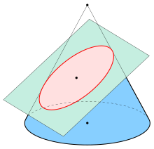
An ellipse (red) obtained as the intersection of a cone with an inclined plane.


Ellipses: examples with increasing eccentricity
In mathematics, an ellipse is a plane curve surrounding two focal points, such that for all points on the curve, the sum of the two distances to the focal points is a constant. It generalizes a circle, which is the special type of ellipse in which the two focal points are the same. The elongation of an ellipse is measured by its eccentricity  , a number ranging from
  (the limiting case of a circle) to
  (the limiting case of infinite elongation, no longer an ellipse but a parabola).
An ellipse has a simple algebraic solution for its area, but only approximations for its perimeter (also known as circumference), for which integration is required to obtain an exact solution.
Analytically, the equation of a standard ellipse centered at the origin with width  and height
  is:
is:

Assuming  , the foci are
  for
for  . The standard parametric equation is:

Ellipses are the closed type of conic section: a plane curve tracing the intersection of a cone with a plane (see figure). Ellipses have many similarities with the other two forms of conic sections, parabolas and hyperbolas, both of which are open and unbounded. An angled cross section of a cylinder is also an ellipse.
An ellipse may also be defined in terms of one focal point and a line outside the ellipse called the directrix: for all points on the ellipse, the ratio between the distance to the focus and the distance to the directrix is a constant. This constant ratio is the above-mentioned eccentricity:

Ellipses are common in physics, astronomy and engineering. For example, the orbit of each planet in the Solar System is approximately an ellipse with the Sun at one focus point (more precisely, the focus is the barycenter of the Sun–planet pair). The same is true for moons orbiting planets and all other systems of two astronomical bodies. The shapes of planets and stars are often well described by ellipsoids. A circle viewed from a side angle looks like an ellipse: that is, the ellipse is the image of a circle under parallel or perspective projection. The ellipse is also the simplest Lissajous figure formed when the horizontal and vertical motions are sinusoids with the same frequency: a similar effect leads to elliptical polarization of light in optics.
The name, ἔλλειψις (élleipsis, «omission»), was given by Apollonius of Perga in his Conics.
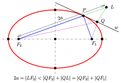
Definition as locus of points[edit]
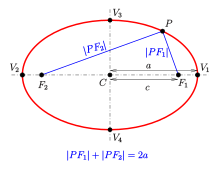
Ellipse: definition by sum of distances to foci
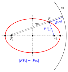
Ellipse: definition by focus and circular directrix
An ellipse can be defined geometrically as a set or locus of points in the Euclidean plane:
- Given two fixed points
 called the foci and a distance which is greater than the distance between the foci, the ellipse is the set of points such that the sum of the distances is equal to :


The midpoint  of the line segment joining the foci is called the center of the ellipse. The line through the foci is called the major axis, and the line perpendicular to it through the center is the minor axis. The major axis intersects the ellipse at two vertices
  , which have distance
  to the center. The distance
  of the foci to the center is called the focal distance or linear eccentricity. The quotient
  is the eccentricity.
The case  yields a circle and is included as a special type of ellipse.
The equation  can be viewed in a different way (see figure):
- If is the circle with center and radius , then the distance of a point to the circle equals the distance to the focus :

 is called the circular directrix (related to focus
  ) of the ellipse.[1][2] This property should not be confused with the definition of an ellipse using a directrix line below.
Using Dandelin spheres, one can prove that any section of a cone with a plane is an ellipse, assuming the plane does not contain the apex and has slope less than that of the lines on the cone.
In Cartesian coordinates[edit]
Shape parameters:
- a: semi-major axis,
- b: semi-minor axis,
- c: linear eccentricity,
- p: semi-latus rectum (usually ).
Standard equation[edit]
The standard form of an ellipse in Cartesian coordinates assumes that the origin is the center of the ellipse, the x-axis is the major axis, and:
- the foci are the points ,
- the major points are .


For an arbitrary point  the distance to the focus
  is
is
 and to the other focus
  . Hence the point
  is on the ellipse whenever:

Removing the radicals by suitable squarings and using  (see diagram) produces the standard equation of the ellipse:[3]

or, solved for y:

The width and height parameters  are called the semi-major and semi-minor axes. The top and bottom points
  are the co-vertices. The distances from a point on the ellipse to the left and right foci are
  and
and  .
.
It follows from the equation that the ellipse is symmetric with respect to the coordinate axes and hence with respect to the origin.
Parameters[edit]
Principal axes[edit]
Throughout this article, the semi-major and semi-minor axes are denoted and  , respectively, i.e.
In principle, the canonical ellipse equation  may have
  (and hence the ellipse would be taller than it is wide). This form can be converted to the standard form by transposing the variable names
  and
and  and the parameter names and
Linear eccentricity[edit]
This is the distance from the center to a focus:  .
.
Eccentricity[edit]
The eccentricity can be expressed as:

assuming  An ellipse with equal axes (
 ) has zero eccentricity, and is a circle.
Semi-latus rectum[edit]
The length of the chord through one focus, perpendicular to the major axis, is called the latus rectum. One half of it is the semi-latus rectum  . A calculation shows:
- [4]

The semi-latus rectum is equal to the radius of curvature at the vertices (see section curvature).
Tangent[edit]
An arbitrary line  intersects an ellipse at 0, 1, or 2 points, respectively called an exterior line, tangent and secant. Through any point of an ellipse there is a unique tangent. The tangent at a point
  of the ellipse has the coordinate equation:

A vector parametric equation of the tangent is:
- with


Proof:
Let be a point on an ellipse and  be the equation of any line containing . Inserting the line’s equation into the ellipse equation and respecting
  yields:

There are then cases:
- Then line and the ellipse have only point in common, and is a tangent. The tangent direction has perpendicular vector , so the tangent line has equation for some . Because is on the tangent and the ellipse, one obtains .
- Then line has a second point in common with the ellipse, and is a secant.


Using (1) one finds that  is a tangent vector at point , which proves the vector equation.
If  and
and  are two points of the ellipse such that
  , then the points lie on two conjugate diameters (see below). (If , the ellipse is a circle and «conjugate» means «orthogonal».)
Shifted ellipse[edit]
If the standard ellipse is shifted to have center  , its equation is

The axes are still parallel to the x- and y-axes.
General ellipse[edit]
In analytic geometry, the ellipse is defined as a quadric: the set of points  of the Cartesian plane that, in non-degenerate cases, satisfy the implicit equation[5][6]

provided 
To distinguish the degenerate cases from the non-degenerate case, let ∆ be the determinant

Then the ellipse is a non-degenerate real ellipse if and only if C∆ < 0. If C∆ > 0, we have an imaginary ellipse, and if ∆ = 0, we have a point ellipse.[7]: p.63
The general equation’s coefficients can be obtained from known semi-major axis , semi-minor axis , center coordinates , and rotation angle  (the angle from the positive horizontal axis to the ellipse’s major axis) using the formulae:
![{displaystyle {begin{aligned}A&=a^{2}sin ^{2}theta +b^{2}cos ^{2}theta \[3mu]B&=2left(b^{2}-a^{2}right)sin theta cos theta \[3mu]C&=a^{2}cos ^{2}theta +b^{2}sin ^{2}theta \[3mu]D&=-2Ax_{circ }-By_{circ }\[3mu]E&=-Bx_{circ }-2Cy_{circ }\[3mu]F&=Ax_{circ }^{2}+Bx_{circ }y_{circ }+Cy_{circ }^{2}-a^{2}b^{2}.end{aligned}}}](https://wikimedia.org/api/rest_v1/media/math/render/svg/0229cbcba4d890d8b7ee7c0bec065a95a2b91229)
These expressions can be derived from the canonical equation

by an affine transformation of the coordinates :

Conversely, the canonical form parameters can be obtained from the general form coefficients by the equations:[citation needed]
![{displaystyle {begin{aligned}a,b&={frac {-{sqrt {2{big (}AE^{2}+CD^{2}-BDE+(B^{2}-4AC)F{big )}{big (}(A+C)pm {sqrt {(A-C)^{2}+B^{2}}}{big )}}}}{B^{2}-4AC}}\x_{circ }&={frac {2CD-BE}{B^{2}-4AC}}\[5mu]y_{circ }&={frac {2AE-BD}{B^{2}-4AC}}\[5mu]theta &={begin{cases}operatorname {arccot} {dfrac {C-A-{sqrt {(A-C)^{2}+B^{2}}}}{B}}&{text{for }}Bneq 0\[5mu]0&{text{for }}B=0, A<C\[10mu]90^{circ }&{text{for }}B=0, A>C\end{cases}}end{aligned}}}](https://wikimedia.org/api/rest_v1/media/math/render/svg/c099e609531d008740862f621a7295d5015a2f9d)
Parametric representation[edit]
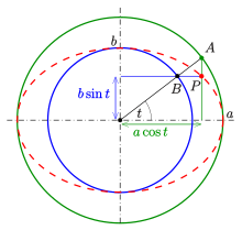
The construction of points based on the parametric equation and the interpretation of parameter t, which is due to de la Hire

Ellipse points calculated by the rational representation with equal spaced parameters ( ).
).
Standard parametric representation[edit]
Using trigonometric functions, a parametric representation of the standard ellipse is:

The parameter t (called the eccentric anomaly in astronomy) is not the angle of  with the x-axis, but has a geometric meaning due to Philippe de La Hire (see Drawing ellipses below).[8]
Rational representation[edit]
With the substitution  and trigonometric formulae one obtains

and the rational parametric equation of an ellipse
![{displaystyle {begin{aligned}x(u)&=a{frac {1-u^{2}}{1+u^{2}}}\[10mu]y(u)&=b{frac {2u}{1+u^{2}}}end{aligned}};,quad -infty <u<infty ;,}](https://wikimedia.org/api/rest_v1/media/math/render/svg/c86f5ffc504dac624df3b6ce483c47521615fd18)
which covers any point of the ellipse except the left vertex  .
.
For ![{displaystyle uin [0,,1],}](https://wikimedia.org/api/rest_v1/media/math/render/svg/c61b780db9ac550dd283876e16abe9c2cccdf8c3) this formula represents the right upper quarter of the ellipse moving counter-clockwise with increasing
this formula represents the right upper quarter of the ellipse moving counter-clockwise with increasing  The left vertex is the limit
Alternately, if the parameter ![{displaystyle [u:v]}](https://wikimedia.org/api/rest_v1/media/math/render/svg/297de5a93c52f13ef84add1d79d693fcda686176) is considered to be a point on the real projective line
is considered to be a point on the real projective line  , then the corresponding rational parametrization is
![{displaystyle [u:v]mapsto left(a{frac {v^{2}-u^{2}}{v^{2}+u^{2}}},b{frac {2uv}{v^{2}+u^{2}}}right).}](https://wikimedia.org/api/rest_v1/media/math/render/svg/fa1c21205522d70966ce62b8e324b19ec4c90f41)
Then ![{textstyle [1:0]mapsto (-a,,0).}](https://wikimedia.org/api/rest_v1/media/math/render/svg/0da12e69b8138a30dcb6cfbeeb95bd63b890f2db)
Rational representations of conic sections are commonly used in computer-aided design (see Bezier curve).
Tangent slope as parameter[edit]
A parametric representation, which uses the slope  of the tangent at a point of the ellipse
can be obtained from the derivative of the standard representation  :
:

With help of trigonometric formulae one obtains:

Replacing  and
and  of the standard representation yields:

Here is the slope of the tangent at the corresponding ellipse point,  is the upper and
  the lower half of the ellipse. The vertices
 , having vertical tangents, are not covered by the representation.
The equation of the tangent at point  has the form
  . The still unknown
  can be determined by inserting the coordinates of the corresponding ellipse point :

This description of the tangents of an ellipse is an essential tool for the determination of the orthoptic of an ellipse. The orthoptic article contains another proof, without differential calculus and trigonometric formulae.
General ellipse[edit]

Ellipse as an affine image of the unit circle
Another definition of an ellipse uses affine transformations:
- Any ellipse is an affine image of the unit circle with equation .

- Parametric representation
An affine transformation of the Euclidean plane has the form  , where
  is a regular matrix (with non-zero determinant) and
  is an arbitrary vector. If
  are the column vectors of the matrix , the unit circle
  ,
,  , is mapped onto the ellipse:

Here is the center and  are the directions of two conjugate diameters, in general not perpendicular.
- Vertices
The four vertices of the ellipse are  , for a parameter
  defined by:

(If  , then
  .) This is derived as follows. The tangent vector at point
  is:
is:

At a vertex parameter , the tangent is perpendicular to the major/minor axes, so:

Expanding and applying the identities  gives the equation for
- Area
From Apollonios theorem (see below) one obtains:
The area of an ellipse  is
is

- Semiaxes
With the abbreviations
 the statements of Apollonios’s theorem can be written as:

Solving this nonlinear system for  yields the semiaxes:


- Implicit representation
Solving the parametric representation for  by Cramer’s rule and using
  , one obtains the implicit representation
- .

Conversely: If the equation
- with


of an ellipse centered at the origin is given, then the two vectors

point to two conjugate points and the tools developed above are applicable.
Example: For the ellipse with equation  the vectors are
- .


Whirls: nested, scaled and rotated ellipses. The spiral is not drawn: we see it as the locus of points where the ellipses are especially close to each other.
- Rotated Standard ellipse
For  one obtains a parametric representation of the standard ellipse rotated by angle :


- Ellipse in space
The definition of an ellipse in this section gives a parametric representation of an arbitrary ellipse, even in space, if one allows  to be vectors in space.
Polar forms[edit]
Polar form relative to center[edit]
Polar coordinates centered at the center.
In polar coordinates, with the origin at the center of the ellipse and with the angular coordinate measured from the major axis, the ellipse’s equation is[7]: p. 75

where is the eccentricity, not Euler’s number
Polar form relative to focus[edit]
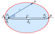
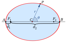
Polar coordinates centered at focus.
If instead we use polar coordinates with the origin at one focus, with the angular coordinate  still measured from the major axis, the ellipse’s equation is

where the sign in the denominator is negative if the reference direction points towards the center (as illustrated on the right), and positive if that direction points away from the center.
In the slightly more general case of an ellipse with one focus at the origin and the other focus at angular coordinate  , the polar form is

The angle in these formulas is called the true anomaly of the point. The numerator of these formulas is the semi-latus rectum  .
.
Eccentricity and the directrix property[edit]
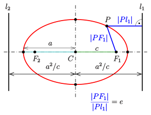
Ellipse: directrix property
Each of the two lines parallel to the minor axis, and at a distance of  from it, is called a directrix of the ellipse (see diagram).
- For an arbitrary point of the ellipse, the quotient of the distance to one focus and to the corresponding directrix (see diagram) is equal to the eccentricity:

The proof for the pair  follows from the fact that
  and
and  satisfy the equation

The second case is proven analogously.
The converse is also true and can be used to define an ellipse (in a manner similar to the definition of a parabola):
- For any point (focus), any line (directrix) not through , and any real number with the ellipse is the locus of points for which the quotient of the distances to the point and to the line is that is:


The extension to , which is the eccentricity of a circle, is not allowed in this context in the Euclidean plane. However, one may consider the directrix of a circle to be the line at infinity in the projective plane.
(The choice yields a parabola, and if  , a hyperbola.)

Pencil of conics with a common vertex and common semi-latus rectum
- Proof
Let  , and assume
  is a point on the curve.
The directrix  has equation
  . With
  , the relation
  produces the equations
- and


The substitution  yields

This is the equation of an ellipse ( ), or a parabola (), or a hyperbola (). All of these non-degenerate conics have, in common, the origin as a vertex (see diagram).
If , introduce new parameters  so that
  , and then the equation above becomes

which is the equation of an ellipse with center  , the x-axis as major axis, and
the major/minor semi axis .

Construction of a directrix
- Construction of a directrix
Because of  point
point  of directrix
  (see diagram) and focus
  are inverse with respect to the circle inversion at circle
  (in diagram green). Hence can be constructed as shown in the diagram. Directrix is the perpendicular to the main axis at point .
- General ellipse
If the focus is  and the directrix
  , one obtains the equation

(The right side of the equation uses the Hesse normal form of a line to calculate the distance  .)
.)
Focus-to-focus reflection property[edit]
Ellipse: the tangent bisects the supplementary angle of the angle between the lines to the foci.
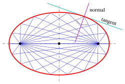
Rays from one focus reflect off the ellipse to pass through the other focus.
An ellipse possesses the following property:
- The normal at a point bisects the angle between the lines .
- Proof
Because the tangent is perpendicular to the normal, the statement is true for the tangent and the supplementary angle of the angle between the lines to the foci (see diagram), too.
Let  be the point on the line
  with the distance to the focus , is the semi-major axis of the ellipse. Let line
  be the bisector of the supplementary angle to the angle between the lines
  . In order to prove that is the tangent line at point
  , one checks that any point
  on line which is different from cannot be on the ellipse. Hence has only point in common with the ellipse and is, therefore, the tangent at point .
From the diagram and the triangle inequality one recognizes that  holds, which means:
  . The equality
  is true from the Angle bisector theorem because
  and
and  . But if is a point of the ellipse, the sum should be .
- Application
The rays from one focus are reflected by the ellipse to the second focus. This property has optical and acoustic applications similar to the reflective property of a parabola (see whispering gallery).
Conjugate diameters[edit]
Definition of conjugate diameters[edit]
Orthogonal diameters of a circle with a square of tangents, midpoints of parallel chords and an affine image, which is an ellipse with conjugate diameters, a parallelogram of tangents and midpoints of chords.
A circle has the following property:
- The midpoints of parallel chords lie on a diameter.
An affine transformation preserves parallelism and midpoints of line segments, so this property is true for any ellipse. (Note that the parallel chords and the diameter are no longer orthogonal.)
- Definition
Two diameters  of an ellipse are conjugate if the midpoints of chords parallel to
  lie on
From the diagram one finds:
- Two diameters of an ellipse are conjugate whenever the tangents at and are parallel to .


Conjugate diameters in an ellipse generalize orthogonal diameters in a circle.
In the parametric equation for a general ellipse given above,

any pair of points  belong to a diameter, and the pair
  belong to its conjugate diameter.
For the common parametric representation  of the ellipse with equation one gets: The points
- (signs: (+,+) or (-,-) )
- (signs: (-,+) or (+,-) )
- are conjugate and


In case of a circle the last equation collapses to 
Theorem of Apollonios on conjugate diameters[edit]


For the alternative area formula
For an ellipse with semi-axes the following is true:[9][10]
- Let and be halves of two conjugate diameters (see diagram) then
- .
- The triangle with sides (see diagram) has the constant area , which can be expressed by , too. is the altitude of point and the angle between the half diameters. Hence the area of the ellipse (see section metric properties) can be written as .
- The parallelogram of tangents adjacent to the given conjugate diameters has the


- Proof
Let the ellipse be in the canonical form with parametric equation
- .

The two points  are on conjugate diameters (see previous section). From trigonometric formulae one obtains
  and
and

The area of the triangle generated by  is
is

and from the diagram it can be seen that the area of the parallelogram is 8 times that of  . Hence
Orthogonal tangents[edit]
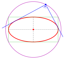
Ellipse with its orthoptic
For the ellipse the intersection points of orthogonal tangents lie on the circle  .
.
This circle is called orthoptic or director circle of the ellipse (not to be confused with the circular directrix defined above).
Drawing ellipses[edit]
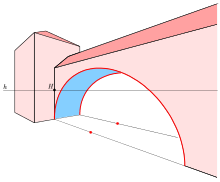
Central projection of circles (gate)
Ellipses appear in descriptive geometry as images (parallel or central projection) of circles. There exist various tools to draw an ellipse. Computers provide the fastest and most accurate method for drawing an ellipse. However, technical tools (ellipsographs) to draw an ellipse without a computer exist. The principle of ellipsographs were known to Greek mathematicians such as Archimedes and Proklos.
If there is no ellipsograph available, one can draw an ellipse using an approximation by the four osculating circles at the vertices.
For any method described below, knowledge of the axes and the semi-axes is necessary (or equivalently: the foci and the semi-major axis).
If this presumption is not fulfilled one has to know at least two conjugate diameters. With help of Rytz’s construction the axes and semi-axes can be retrieved.
de La Hire’s point construction[edit]
The following construction of single points of an ellipse is due to de La Hire.[11] It is based on the standard parametric representation  of an ellipse:
- Draw the two circles centered at the center of the ellipse with radii and the axes of the ellipse.
- Draw a line through the center, which intersects the two circles at point and , respectively.
- Draw a line through that is parallel to the minor axis and a line through that is parallel to the major axis. These lines meet at an ellipse point (see diagram).
- Repeat steps (2) and (3) with different lines through the center.

-

de La Hire’s method
-

Animation of the method
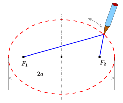
Ellipse: gardener’s method
Pins-and-string method[edit]
The characterization of an ellipse as the locus of points so that sum of the distances to the foci is constant leads to a method of drawing one using two drawing pins, a length of string, and a pencil. In this method, pins are pushed into the paper at two points, which become the ellipse’s foci. A string is tied at each end to the two pins; its length after tying is . The tip of the pencil then traces an ellipse if it is moved while keeping the string taut. Using two pegs and a rope, gardeners use this procedure to outline an elliptical flower bed—thus it is called the gardener’s ellipse.
A similar method for drawing confocal ellipses with a closed string is due to the Irish bishop Charles Graves.
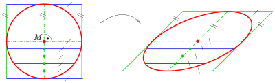
Paper strip methods[edit]
The two following methods rely on the parametric representation (see section parametric representation, above):
This representation can be modeled technically by two simple methods. In both cases center, the axes and semi axes have to be known.
- Method 1
The first method starts with
- a strip of paper of length .
The point, where the semi axes meet is marked by . If the strip slides with both ends on the axes of the desired ellipse, then point traces the ellipse. For the proof one shows that point has the parametric representation , where parameter  is the angle of the slope of the paper strip.
A technical realization of the motion of the paper strip can be achieved by a Tusi couple (see animation). The device is able to draw any ellipse with a fixed sum  , which is the radius of the large circle. This restriction may be a disadvantage in real life. More flexible is the second paper strip method.
-

Ellipse construction: paper strip method 1
-

Ellipses with Tusi couple. Two examples: red and cyan.


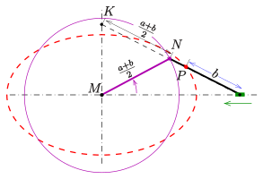
A variation of the paper strip method 1 uses the observation that the midpoint  of the paper strip is moving on the circle with center
  (of the ellipse) and radius
  . Hence, the paperstrip can be cut at point into halves, connected again by a joint at and the sliding end
  fixed at the center (see diagram). After this operation the movement of the unchanged half of the paperstrip is unchanged.[12] This variation requires only one sliding shoe.
-

Variation of the paper strip method 1
-

Animation of the variation of the paper strip method 1


Ellipse construction: paper strip method 2
- Method 2
The second method starts with
- a strip of paper of length .
One marks the point, which divides the strip into two substrips of length and  . The strip is positioned onto the axes as described in the diagram. Then the free end of the strip traces an ellipse, while the strip is moved. For the proof, one recognizes that the tracing point can be described parametrically by , where parameter is the angle of slope of the paper strip.
This method is the base for several ellipsographs (see section below).
Similar to the variation of the paper strip method 1 a variation of the paper strip method 2 can be established (see diagram) by cutting the part between the axes into halves.
-

-

Variation of the paper strip method 2
Most ellipsograph drafting instruments are based on the second paperstrip method.
Approximation of an ellipse with osculating circles
Approximation by osculating circles[edit]
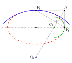
From Metric properties below, one obtains:
The diagram shows an easy way to find the centers of curvature  at vertex
  and co-vertex
  , respectively:
- mark the auxiliary point and draw the line segment
- draw the line through , which is perpendicular to the line
- the intersection points of this line with the axes are the centers of the osculating circles.


(proof: simple calculation.)
The centers for the remaining vertices are found by symmetry.
With help of a French curve one draws a curve, which has smooth contact to the osculating circles.
Steiner generation[edit]

Ellipse: Steiner generation
Ellipse: Steiner generation
The following method to construct single points of an ellipse relies on the Steiner generation of a conic section:
- Given two pencils of lines at two points (all lines containing and , respectively) and a projective but not perspective mapping of onto , then the intersection points of corresponding lines form a non-degenerate projective conic section.


For the generation of points of the ellipse one uses the pencils at the vertices  . Let
. Let  be an upper co-vertex of the ellipse and
  .
.
is the center of the rectangle  . The side
  of the rectangle is divided into n equal spaced line segments and this division is projected parallel with the diagonal
  as direction onto the line segment
  and assign the division as shown in the diagram. The parallel projection together with the reverse of the orientation is part of the projective mapping between the pencils at and
  needed. The intersection points of any two related lines
  and
and  are points of the uniquely defined ellipse. With help of the points
  the points of the second quarter of the ellipse can be determined. Analogously one obtains the points of the lower half of the ellipse.
Steiner generation can also be defined for hyperbolas and parabolas. It is sometimes called a parallelogram method because one can use other points rather than the vertices, which starts with a parallelogram instead of a rectangle.
As hypotrochoid[edit]
An ellipse (in red) as a special case of the hypotrochoid with R = 2r
The ellipse is a special case of the hypotrochoid when  , as shown in the adjacent image. The special case of a moving circle with radius
  inside a circle with radius is called a Tusi couple.
Inscribed angles and three-point form[edit]
Circles[edit]
Circle: inscribed angle theorem
A circle with equation  is uniquely determined by three points
  not on a line. A simple way to determine the parameters
  uses the inscribed angle theorem for circles:
- For four points (see diagram) the following statement is true:
- The four points are on a circle if and only if the angles at and are equal.


Usually one measures inscribed angles by a degree or radian θ, but here the following measurement is more convenient:
- In order to measure the angle between two lines with equations one uses the quotient:


Inscribed angle theorem for circles[edit]
For four points  no three of them on a line, we have the following (see diagram):
- The four points are on a circle, if and only if the angles at and are equal. In terms of the angle measurement above, this means:

At first the measure is available only for chords not parallel to the y-axis, but the final formula works for any chord.
Three-point form of circle equation[edit]
- As a consequence, one obtains an equation for the circle determined by three non-colinear points :


For example, for  the three-point equation is:
- , which can be rearranged to


Using vectors, dot products and determinants this formula can be arranged more clearly, letting  :
:

The center of the circle satisfies:

The radius is the distance between any of the three points and the center.

Ellipses[edit]
This section, we consider the family of ellipses defined by equations  with a fixed eccentricity . It is convenient to use the parameter:

and to write the ellipse equation as:

where q is fixed and  vary over the real numbers. (Such ellipses have their axes parallel to the coordinate axes: if
  , the major axis is parallel to the x-axis; if
  , it is parallel to the y-axis.)

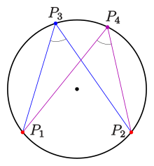
Inscribed angle theorem for an ellipse
Like a circle, such an ellipse is determined by three points not on a line.
For this family of ellipses, one introduces the following q-analog angle measure, which is not a function of the usual angle measure θ:[13][14]
- In order to measure an angle between two lines with equations one uses the quotient:


Inscribed angle theorem for ellipses[edit]
- Given four points , no three of them on a line (see diagram).
- The four points are on an ellipse with equation if and only if the angles at and are equal in the sense of the measurement above—that is, if


At first the measure is available only for chords which are not parallel to the y-axis. But the final formula works for any chord. The proof follows from a straightforward calculation. For the direction of proof given that the points are on an ellipse, one can assume that the center of the ellipse is the origin.
Three-point form of ellipse equation[edit]
- A consequence, one obtains an equation for the ellipse determined by three non-colinear points :

For example, for and  one obtains the three-point form
- and after conversion


Analogously to the circle case, the equation can be written more clearly using vectors:

where  is the modified dot product
Pole-polar relation[edit]
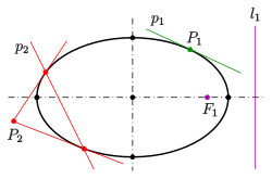
Ellipse: pole-polar relation
Any ellipse can be described in a suitable coordinate system by an equation . The equation of the tangent at a point  of the ellipse is
  If one allows point to be an arbitrary point different from the origin, then
- point is mapped onto the line , not through the center of the ellipse.


This relation between points and lines is a bijection.
The inverse function maps
Such a relation between points and lines generated by a conic is called pole-polar relation or polarity. The pole is the point; the polar the line.
By calculation one can confirm the following properties of the pole-polar relation of the ellipse:
- The intersection point of two polars is the pole of the line through their poles.
- The foci and , respectively, and the directrices and , respectively, belong to pairs of pole and polar. Because they are even polar pairs with respect to the circle , the directrices can be constructed by compass and straightedge (see Inversive geometry).


Pole-polar relations exist for hyperbolas and parabolas as well.
Metric properties[edit]
All metric properties given below refer to an ellipse with equation
-
(1)
except for the section on the area enclosed by a tilted ellipse, where the generalized form of Eq.(1) will be given.
Area[edit]
The area  enclosed by an ellipse is:
-
(2)

where and are the lengths of the semi-major and semi-minor axes, respectively. The area formula  is intuitive: start with a circle of radius (so its area is
  ) and stretch it by a factor
  to make an ellipse. This scales the area by the same factor:
  [15] However, using the same approach for the circumference would be fallacious – compare the integrals
  and
and  . It is also easy to rigorously prove the area formula using integration as follows. Equation (1) can be rewritten as
  For
For ![{displaystyle xin [-a,a],}](https://wikimedia.org/api/rest_v1/media/math/render/svg/fb19e5015712fa6f6c57d3f334266c73d7782434) this curve is the top half of the ellipse. So twice the integral of
this curve is the top half of the ellipse. So twice the integral of  over the interval
 ![[-a,a]](https://wikimedia.org/api/rest_v1/media/math/render/svg/50ccbcece37f9ec0a4c6d396be3a143a0b76d5c1) will be the area of the ellipse:
will be the area of the ellipse:

The second integral is the area of a circle of radius  that is,
  So
So

An ellipse defined implicitly by  has area
The area can also be expressed in terms of eccentricity and the length of the semi-major axis as  (obtained by solving for flattening, then computing the semi-minor axis).
The area enclosed by a tilted ellipse is  .
.
So far we have dealt with erect ellipses, whose major and minor axes are parallel to the and axes. However, some applications require tilted ellipses. In charged-particle beam optics, for instance, the enclosed area of an erect or tilted ellipse is an important property of the beam, its emittance. In this case a simple formula still applies, namely
-
(3)

where  ,
,  are intercepts and
  ,
,  are maximum values. It follows directly from Apollonios’s theorem.
Circumference[edit]

Ellipses with same circumference
The circumference of an ellipse is:

where again is the length of the semi-major axis,  is the eccentricity, and the function
  is the complete elliptic integral of the second kind,

which is in general not an elementary function.
The circumference of the ellipse may be evaluated in terms of  using Gauss’s arithmetic-geometric mean;[16] this is a quadratically converging iterative method (see here for details).
The exact infinite series is:
![{displaystyle {begin{aligned}C&=2pi aleft[{1-left({frac {1}{2}}right)^{2}e^{2}-left({frac {1cdot 3}{2cdot 4}}right)^{2}{frac {e^{4}}{3}}-left({frac {1cdot 3cdot 5}{2cdot 4cdot 6}}right)^{2}{frac {e^{6}}{5}}-cdots }right]\&=2pi aleft[1-sum _{n=1}^{infty }left({frac {(2n-1)!!}{(2n)!!}}right)^{2}{frac {e^{2n}}{2n-1}}right]\&=-2pi asum _{n=0}^{infty }left({frac {(2n-1)!!}{(2n)!!}}right)^{2}{frac {e^{2n}}{2n-1}},end{aligned}}}](https://wikimedia.org/api/rest_v1/media/math/render/svg/3e202a234c19a28620ecf9c6d260eb21b1bd7aa0)
where  is the double factorial (extended to negative odd integers by the recurrence relation
  , for
, for  ). This series converges, but by expanding in terms of
  James Ivory[17] and Bessel[18] derived an expression that converges much more rapidly:
![{displaystyle {begin{aligned}C&=pi (a+b)sum _{n=0}^{infty }left({frac {(2n-3)!!}{2^{n}n!}}right)^{2}h^{n}\&=pi (a+b)left[1+{frac {h}{4}}+sum _{n=2}^{infty }left({frac {(2n-3)!!}{2^{n}n!}}right)^{2}h^{n}right]\&=pi (a+b)left[1+sum _{n=1}^{infty }left({frac {(2n-1)!!}{2^{n}n!}}right)^{2}{frac {h^{n}}{(2n-1)^{2}}}right].end{aligned}}}](https://wikimedia.org/api/rest_v1/media/math/render/svg/7d29d8f31216e5d32400e99b04e75e242d987893)
Srinivasa Ramanujan gave two close approximations for the circumference in §16 of «Modular Equations and Approximations to  «;[19] they are
![{displaystyle Capprox pi {biggl [}3(a+b)-{sqrt {(3a+b)(a+3b)}}{biggr ]}=pi {biggl [}3(a+b)-{sqrt {10ab+3left(a^{2}+b^{2}right)}}{biggr ]}}](https://wikimedia.org/api/rest_v1/media/math/render/svg/86c8a7234c16af19a7338faafe61b4cf9a333f80)
and

where  takes on the same meaning as above. The errors in these approximations, which were obtained empirically, are of order
  and
and  respectively.
Arc length[edit]
More generally, the arc length of a portion of the circumference, as a function of the angle subtended (or x coordinates of any two points on the upper half of the ellipse), is given by an incomplete elliptic integral. The upper half of an ellipse is parameterized by

Then the arc length  from
from  to
to  is:
is:

This is equivalent to
![{displaystyle s=b left[;Eleft(z;{Biggl |};1-{frac {a^{2}}{b^{2}}}right);right]_{z = arccos {frac {x_{2}}{a}}}^{arccos {frac {x_{1}}{a}}}}](https://wikimedia.org/api/rest_v1/media/math/render/svg/b7338c6c7bf9cc8e20da6c7da90eecd93f540416)
where  is the incomplete elliptic integral of the second kind with parameter
Some lower and upper bounds on the circumference of the canonical ellipse  with
with  are[20]

Here the upper bound  is the circumference of a circumscribed concentric circle passing through the endpoints of the ellipse’s major axis, and the lower bound
  is the perimeter of an inscribed rhombus with vertices at the endpoints of the major and the minor axes.
Curvature[edit]
The curvature is given by 
radius of curvature at point :

Radius of curvature at the two vertices  and the centers of curvature:

Radius of curvature at the two co-vertices  and the centers of curvature:

In triangle geometry[edit]
Ellipses appear in triangle geometry as
- Steiner ellipse: ellipse through the vertices of the triangle with center at the centroid,
- inellipses: ellipses which touch the sides of a triangle. Special cases are the Steiner inellipse and the Mandart inellipse.
As plane sections of quadrics[edit]
Ellipses appear as plane sections of the following quadrics:
- Ellipsoid
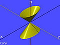
- Elliptic cone
- Elliptic cylinder
- Hyperboloid of one sheet
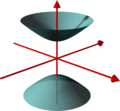
- Hyperboloid of two sheets
-

Ellipsoid
-

Elliptic cone
-
Elliptic cylinder
-

Hyperboloid of one sheet
-

Hyperboloid of two sheets


Applications[edit]
Physics[edit]
Elliptical reflectors and acoustics[edit]

Wave pattern of a little droplet dropped into mercury in one focus of the ellipse
If the water’s surface is disturbed at one focus of an elliptical water tank, the circular waves of that disturbance, after reflecting off the walls, converge simultaneously to a single point: the second focus. This is a consequence of the total travel length being the same along any wall-bouncing path between the two foci.
Similarly, if a light source is placed at one focus of an elliptic mirror, all light rays on the plane of the ellipse are reflected to the second focus. Since no other smooth curve has such a property, it can be used as an alternative definition of an ellipse. (In the special case of a circle with a source at its center all light would be reflected back to the center.) If the ellipse is rotated along its major axis to produce an ellipsoidal mirror (specifically, a prolate spheroid), this property holds for all rays out of the source. Alternatively, a cylindrical mirror with elliptical cross-section can be used to focus light from a linear fluorescent lamp along a line of the paper; such mirrors are used in some document scanners.
Sound waves are reflected in a similar way, so in a large elliptical room a person standing at one focus can hear a person standing at the other focus remarkably well. The effect is even more evident under a vaulted roof shaped as a section of a prolate spheroid. Such a room is called a whisper chamber. The same effect can be demonstrated with two reflectors shaped like the end caps of such a spheroid, placed facing each other at the proper distance. Examples are the National Statuary Hall at the United States Capitol (where John Quincy Adams is said to have used this property for eavesdropping on political matters); the Mormon Tabernacle at Temple Square in Salt Lake City, Utah; at an exhibit on sound at the Museum of Science and Industry in Chicago; in front of the University of Illinois at Urbana–Champaign Foellinger Auditorium; and also at a side chamber of the Palace of Charles V, in the Alhambra.
Planetary orbits[edit]
In the 17th century, Johannes Kepler discovered that the orbits along which the planets travel around the Sun are ellipses with the Sun [approximately] at one focus, in his first law of planetary motion. Later, Isaac Newton explained this as a corollary of his law of universal gravitation.
More generally, in the gravitational two-body problem, if the two bodies are bound to each other (that is, the total energy is negative), their orbits are similar ellipses with the common barycenter being one of the foci of each ellipse. The other focus of either ellipse has no known physical significance. The orbit of either body in the reference frame of the other is also an ellipse, with the other body at the same focus.
Keplerian elliptical orbits are the result of any radially directed attraction force whose strength is inversely proportional to the square of the distance. Thus, in principle, the motion of two oppositely charged particles in empty space would also be an ellipse. (However, this conclusion ignores losses due to electromagnetic radiation and quantum effects, which become significant when the particles are moving at high speed.)
For elliptical orbits, useful relations involving the eccentricity are:

where
Also, in terms of  and
and  , the semi-major axis is their arithmetic mean, the semi-minor axis is their geometric mean, and the semi-latus rectum is their harmonic mean. In other words,
- .
![{displaystyle {begin{aligned}a&={frac {r_{a}+r_{p}}{2}}\[2pt]b&={sqrt {r_{a}r_{p}}}\[2pt]ell &={frac {2}{{frac {1}{r_{a}}}+{frac {1}{r_{p}}}}}={frac {2r_{a}r_{p}}{r_{a}+r_{p}}}end{aligned}}}](https://wikimedia.org/api/rest_v1/media/math/render/svg/08835a73be73e7094f529d4eff42804930898271)
Harmonic oscillators[edit]
The general solution for a harmonic oscillator in two or more dimensions is also an ellipse. Such is the case, for instance, of a long pendulum that is free to move in two dimensions; of a mass attached to a fixed point by a perfectly elastic spring; or of any object that moves under influence of an attractive force that is directly proportional to its distance from a fixed attractor. Unlike Keplerian orbits, however, these «harmonic orbits» have the center of attraction at the geometric center of the ellipse, and have fairly simple equations of motion.
Phase visualization[edit]
In electronics, the relative phase of two sinusoidal signals can be compared by feeding them to the vertical and horizontal inputs of an oscilloscope. If the Lissajous figure display is an ellipse, rather than a straight line, the two signals are out of phase.
Elliptical gears[edit]
Two non-circular gears with the same elliptical outline, each pivoting around one focus and positioned at the proper angle, turn smoothly while maintaining contact at all times. Alternatively, they can be connected by a link chain or timing belt, or in the case of a bicycle the main chainring may be elliptical, or an ovoid similar to an ellipse in form. Such elliptical gears may be used in mechanical equipment to produce variable angular speed or torque from a constant rotation of the driving axle, or in the case of a bicycle to allow a varying crank rotation speed with inversely varying mechanical advantage.
Elliptical bicycle gears make it easier for the chain to slide off the cog when changing gears.[21]
An example gear application would be a device that winds thread onto a conical bobbin on a spinning machine. The bobbin would need to wind faster when the thread is near the apex than when it is near the base.[22]
Optics[edit]
- In a material that is optically anisotropic (birefringent), the refractive index depends on the direction of the light. The dependency can be described by an index ellipsoid. (If the material is optically isotropic, this ellipsoid is a sphere.)
- In lamp-pumped solid-state lasers, elliptical cylinder-shaped reflectors have been used to direct light from the pump lamp (coaxial with one ellipse focal axis) to the active medium rod (coaxial with the second focal axis).[23]
- In laser-plasma produced EUV light sources used in microchip lithography, EUV light is generated by plasma positioned in the primary focus of an ellipsoid mirror and is collected in the secondary focus at the input of the lithography machine.[24]
Statistics and finance[edit]
In statistics, a bivariate random vector  is jointly elliptically distributed if its iso-density contours—loci of equal values of the density function—are ellipses. The concept extends to an arbitrary number of elements of the random vector, in which case in general the iso-density contours are ellipsoids. A special case is the multivariate normal distribution. The elliptical distributions are important in finance because if rates of return on assets are jointly elliptically distributed then all portfolios can be characterized completely by their mean and variance—that is, any two portfolios with identical mean and variance of portfolio return have identical distributions of portfolio return.[25][26]
Computer graphics[edit]
Drawing an ellipse as a graphics primitive is common in standard display libraries, such as the MacIntosh QuickDraw API, and Direct2D on Windows. Jack Bresenham at IBM is most famous for the invention of 2D drawing primitives, including line and circle drawing, using only fast integer operations such as addition and branch on carry bit. M. L. V. Pitteway extended Bresenham’s algorithm for lines to conics in 1967.[27] Another efficient generalization to draw ellipses was invented in 1984 by Jerry Van Aken.[28]
In 1970 Danny Cohen presented at the «Computer Graphics 1970» conference in England a linear algorithm for drawing ellipses and circles. In 1971, L. B. Smith published similar algorithms for all conic sections and proved them to have good properties.[29] These algorithms need only a few multiplications and additions to calculate each vector.
It is beneficial to use a parametric formulation in computer graphics because the density of points is greatest where there is the most curvature. Thus, the change in slope between each successive point is small, reducing the apparent «jaggedness» of the approximation.
- Drawing with Bézier paths
Composite Bézier curves may also be used to draw an ellipse to sufficient accuracy, since any ellipse may be construed as an affine transformation of a circle. The spline methods used to draw a circle may be used to draw an ellipse, since the constituent Bézier curves behave appropriately under such transformations.
Optimization theory[edit]
It is sometimes useful to find the minimum bounding ellipse on a set of points. The ellipsoid method is quite useful for solving this problem.
See also[edit]
- Cartesian oval, a generalization of the ellipse
- Circumconic and inconic
- Distance of closest approach of ellipses
- Ellipse fitting
- Elliptic coordinates, an orthogonal coordinate system based on families of ellipses and hyperbolae
- Elliptic partial differential equation
- Elliptical distribution, in statistics
- Elliptical dome
- Geodesics on an ellipsoid
- Great ellipse
- Kepler’s laws of planetary motion
- n-ellipse, a generalization of the ellipse for n foci
- Oval
- Spheroid, the ellipsoid obtained by rotating an ellipse about its major or minor axis
- Stadium (geometry), a two-dimensional geometric shape constructed of a rectangle with semicircles at a pair of opposite sides
- Steiner circumellipse, the unique ellipse circumscribing a triangle and sharing its centroid
- Superellipse, a generalization of an ellipse that can look more rectangular or more «pointy»
- True, eccentric, and mean anomaly
Notes[edit]
- ^ Apostol, Tom M.; Mnatsakanian, Mamikon A. (2012), New Horizons in Geometry, The Dolciani Mathematical Expositions #47, The Mathematical Association of America, p. 251, ISBN 978-0-88385-354-2
- ^ The German term for this circle is Leitkreis which can be translated as «Director circle», but that term has a different meaning in the English literature (see Director circle).
- ^ «Ellipse — from Wolfram MathWorld». Mathworld.wolfram.com. 2020-09-10. Retrieved 2020-09-10.
- ^ Protter & Morrey (1970, pp. 304, APP-28)
- ^ Larson, Ron; Hostetler, Robert P.; Falvo, David C. (2006). «Chapter 10». Precalculus with Limits. Cengage Learning. p. 767. ISBN 978-0-618-66089-6.
- ^ Young, Cynthia Y. (2010). «Chapter 9». Precalculus. John Wiley and Sons. p. 831. ISBN 978-0-471-75684-2.
- ^ a b Lawrence, J. Dennis, A Catalog of Special Plane Curves, Dover Publ., 1972.
- ^ K. Strubecker: Vorlesungen über Darstellende Geometrie, GÖTTINGEN,
VANDENHOECK & RUPRECHT, 1967, p. 26 - ^ Bronstein&Semendjajew: Taschenbuch der Mathematik, Verlag Harri Deutsch, 1979, ISBN 3871444928, p. 274.
- ^ Encyclopedia of Mathematics, Springer, URL: http://encyclopediaofmath.org/index.php?title=Apollonius_theorem&oldid=17516 .
- ^ K. Strubecker: Vorlesungen über Darstellende Geometrie. Vandenhoeck & Ruprecht, Göttingen 1967, S. 26.
- ^ J. van Mannen: Seventeenth century instruments for drawing conic sections. In: The Mathematical Gazette. Vol. 76, 1992, p. 222–230.
- ^ E. Hartmann: Lecture Note ‘Planar Circle Geometries’, an Introduction to Möbius-, Laguerre- and Minkowski Planes, p. 55
- ^ W. Benz, Vorlesungen über Geomerie der Algebren, Springer (1973)
- ^ Archimedes. (1897). The works of Archimedes. Heath, Thomas Little, Sir, 1861-1940. Mineola, N.Y.: Dover Publications. p. 115. ISBN 0-486-42084-1. OCLC 48876646.
- ^ Carlson, B. C. (2010), «Elliptic Integrals», in Olver, Frank W. J.; Lozier, Daniel M.; Boisvert, Ronald F.; Clark, Charles W. (eds.), NIST Handbook of Mathematical Functions, Cambridge University Press, ISBN 978-0-521-19225-5, MR 2723248
- ^ Ivory, J. (1798). «A new series for the rectification of the ellipsis». Transactions of the Royal Society of Edinburgh. 4 (2): 177–190. doi:10.1017/s0080456800030817. S2CID 251572677.
- ^ Bessel, F. W. (2010). «The calculation of longitude and latitude from geodesic measurements (1825)». Astron. Nachr. 331 (8): 852–861. arXiv:0908.1824. Bibcode:2010AN….331..852K. doi:10.1002/asna.201011352. S2CID 118760590. Englisch translation of Bessel, F. W. (1825). «Über die Berechnung der geographischen Längen und Breiten aus geodätischen Vermesssungen». Astron. Nachr. 4 (16): 241–254. arXiv:0908.1823. Bibcode:1825AN……4..241B. doi:10.1002/asna.18260041601. S2CID 118630614.
- ^ Ramanujan, Srinivasa (1914). «Modular Equations and Approximations to π». Quart. J. Pure App. Math. 45: 350–372. ISBN 9780821820766.
- ^ Jameson, G.J.O. (2014). «Inequalities for the perimeter of an ellipse». Mathematical Gazette. 98 (542): 227–234. doi:10.1017/S002555720000125X. S2CID 125063457.
- ^ David Drew.
«Elliptical Gears».
[1] - ^ Grant, George B. (1906). A treatise on gear wheels. Philadelphia Gear Works. p. 72.
- ^ Encyclopedia of Laser Physics and Technology — lamp-pumped lasers, arc lamps, flash lamps, high-power, Nd:YAG laser
- ^ «Cymer — EUV Plasma Chamber Detail Category Home Page». Archived from the original on 2013-05-17. Retrieved 2013-06-20.
- ^ Chamberlain, G. (February 1983). «A characterization of the distributions that imply mean—Variance utility functions». Journal of Economic Theory. 29 (1): 185–201. doi:10.1016/0022-0531(83)90129-1.
- ^ Owen, J.; Rabinovitch, R. (June 1983). «On the class of elliptical distributions and their applications to the theory of portfolio choice». Journal of Finance. 38 (3): 745–752. doi:10.1111/j.1540-6261.1983.tb02499.x. JSTOR 2328079.
- ^ Pitteway, M.L.V. (1967). «Algorithm for drawing ellipses or hyperbolae with a digital plotter». The Computer Journal. 10 (3): 282–9. doi:10.1093/comjnl/10.3.282.
- ^ Van Aken, J.R. (September 1984). «An Efficient Ellipse-Drawing Algorithm». IEEE Computer Graphics and Applications. 4 (9): 24–35. doi:10.1109/MCG.1984.275994. S2CID 18995215.
- ^ Smith, L.B. (1971). «Drawing ellipses, hyperbolae or parabolae with a fixed number of points». The Computer Journal. 14 (1): 81–86. doi:10.1093/comjnl/14.1.81.
References[edit]
- Besant, W.H. (1907). «Chapter III. The Ellipse». Conic Sections. London: George Bell and Sons. p. 50.
- Coxeter, H.S.M. (1969). Introduction to Geometry (2nd ed.). New York: Wiley. pp. 115–9.
- Meserve, Bruce E. (1983) [1959], Fundamental Concepts of Geometry, Dover Publications, ISBN 978-0-486-63415-9
- Miller, Charles D.; Lial, Margaret L.; Schneider, David I. (1990). Fundamentals of College Algebra (3rd ed.). Scott Foresman/Little. p. 381. ISBN 978-0-673-38638-0.
- Protter, Murray H.; Morrey, Charles B. Jr. (1970), College Calculus with Analytic Geometry (2nd ed.), Reading: Addison-Wesley, LCCN 76087042
External links[edit]
Эллипс – это замкнутая плоская кривая, сумма расстояний от каждой точки до двух точек равняется постоянной величине.
Что такое эллипс и фокусное расстояние
Эллипс – это множество точек плоскости, сумма расстояний которых от двух заданных точек, что называются фокусами, есть постоянная величина и равна  .
.
Обозначим фокусы эллипса  и
и  . Допустим, что расстояние
  =
=  – фокусное расстояние.
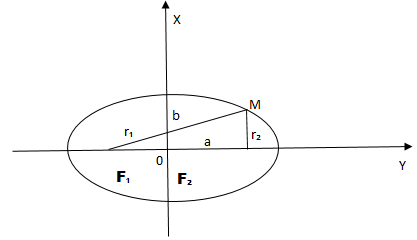
Рис. 1
 – фокусы .
 ;
;  ,
,
 – половина расстояния между фокусами;
 – большая полуось;
 – малая полуось.
Теорема:
Фокусное расстояние и полуоси связаны соотношением:

Если точка  находится на пересечении эллипса с вертикальной осью,
  (теорема Пифагора). Если же точка находится на пересечении его с горизонтальной осью,
  . Так как по определению сумма
  – постоянная величина, то приравнивая получается:
 .
.
Уравнение эллипса
Уравнение элиппса бывает двух видов:
- Каноническое уравнение эллипса.
- Параметрическое уравнение эллипса.
Сначала рассмотрим каноническое уравнение эллипса:
Уравнение описывает эллипс в декартовой системе координат. Если центр эллипсa  в начале системы координат, а большая ось лежит на абсциссе, то эллипс описывается уравнением:

Если центр эллипсa смещен в точку с координатами  тогда уравнение:

Чтобы получить каноническое уравнение эллипса, разместим и на оси  симметричной к началу координат. Тогда у фокусов будут такие координаты
  и
и  (см. рис. 2).
Пусть  – произвольная точка эллипса. Обозначим через
  и
и  – расстояние от точки к фокусам. Согласно с определением эллипса:

(1)
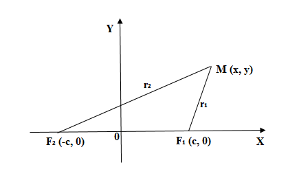
Рис. 2
Подставим в (1)  ,
,  и освободимся от иррациональности, подняв обе части к квадрату, получим:


(подносим к квадрату обе части):  ,
,

Обозначим:  , получаем каноническое уравнение эллипса:

(2)
Отметим, что по известному свойству треугольника (сумма двух сторон больше третьей) из  у нас получается
  . Так как , тогда
  , и поэтому
  .
.
Для построения эллипса обратим внимание, что если точка  принадлежит эллипсу, то есть удовлетворяет уравнение (2), тогда точки
  тоже удовлетворяют это уравнение: из
 .
.
Точки  – расположены симметрично относительно осей координат. Значит, эллипс – фигура, симметричная относительно координатных осей. Поэтому достаточно построить график в первой четверти, а тогда симметрично продолжить его.
Из уравнения (2) находим  , для первой четверти
  .
.
Если  , тогда
  . Если же
  , тогда
  . Точки
  и
и  , а также симметричные с ними
  ,
,  – вершины эллипса, точка
  – центр эллипса,
  =
=  большая ось,
  – малая ось эллипса.
Если  первой четверти, тогда из
  получается, что при возрастании
  от
от  к значение
  падает от к . (рис. 3)
Параметрическое уравнение выглядит так:

Основные свойства эллипса
Рассмотрим основные свойства эллипса, которые необходимы для решения многих задач.
1. Угол между касательной к эллипсу и фокальным радиусом равен углу между касательной и фокальным радиусом .
2. Уравнение касательной к эллипсу в точке с координатами  :
:
 .
.
3. Если эллипс пересекается двумя параллельными прямыми, то отрезок, который соединяет середины отрезков образовавшихся при пересечении прямых и эллипса, всегда проходит через середину (центр) эллипсa. (При помощи данного свойства можно построить эллипс при помощи циркуля и линейка, а также найти центр эллипса).
4. Эволюта эллипсa – это астероида, которая растянута вдоль короткой оси.
5. Если вписать эллипс с фокусами и у треугольника  , тогда выполняется соотношение:
 =
= 
Эксцентриситет эллипса
Эксентриситет эллипса – это величина отношения межфокусного расстояния к большей оси и после сокращения на  обозначается
Значения эксентриситета характеризует степень “сплющенность” эллипса. Если  , тогда
  – получается круг. Если же
  , тогда
  – эллипс превращается в отрезок. В некоторых случаях
  . Для фокальных радиусов приведём без доказательства такие формулы:
![left{ begin{aligned} r_{1} = a - varepsilon{x},\ r_{2} = a + varepsilon, end{aligned} quad{xin[-a, a]. right](https://nauchniestati.ru/wp-content/ql-cache/quicklatex.com-4ceb6a00f3ad3e56a309592ec9432bd2_l3.svg "Rendered by QuickLaTeX.com")
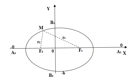
Рис. 3
Эллипс можно построить механическим способом. Из канонического уравнения нужно найти полуоси и , тогда вычислим  – полуфокусное расстояние.
Строим фокусы и на расстоянии один от другого Концы не растянутой нити длиной закрепляем в точках и . Натягивая остриём карандаша нитку, водим остриём по плоскости таким образом, чтобы нитка скользила по острию. Карандаш при этом опишет полуось. Оттягивая нить в противоположную сторону, начертим вторую половину эллипса.
Примеры решения задач
Задача
Задан эллипс уравнением  и точки
  . Необходимо:
- убедиться, что точки
 и
и  лежат на эллипсе;
 - найти полуоси эллипса и координаты его фокусов;
- найти расстояние от точки к фокусам;
- убедиться, что сумма этих расстояний равна длине большой оси;
- найти эксентриситет эллипса.
Решение
1. Подставим координаты  точки
точки  в левую часть уравнения эллипса:
 – точка лежит на эллипсе. Аналогично для
  :
:
 точка
точка  лежит на эллипсе.
2. С канонического и данного уравнения эллипса выходит:  Из равенства
  получается:
 – полуфокусное расстояние. Координаты фокусов
  и
и  .
.
3. Найдём фокальные радиусы точки :


4. Найдём сумму  , что отвечает определению эллипса.
5. Эксцентриситет находится по формуле  .
.
Задача
Найти оси, вершины и фокусы эллипса 
Решение
Сведём обычное уравнение к каноническому:

 ,
,  . Вершины эллипса в точках
  ,
,  ,
,  ,
,  . Строим вершины на координатных осях и соединяем плавной линией (см. рис. 2). Так как в данном случае
  больше, чем
  , то эллипс, который вытянут вдоль оси
  , находим полуфокусное расстояние
  .
.
Фокусы в точках  и
и  . (см. рис. 3)
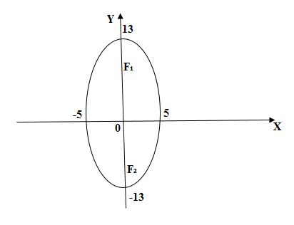
Рис. 4
Найти оси, вершины и фокусы эллипса  или
или  . Построить эллипс.
Сравнивая последнее уравнение с уравнением (2), у нас получается:
 ,
,  . Откуда находим оси эллипса:
  ,
,  и координаты вершин:
  ,
,  ,
,  ,
,  . Дальше из формулы:
 . Значит, фокусами эллипса есть точки:
  и
и  . Для построения эллипса отложим на осях и вершины
  соответственно соединим их плавной линией, (см. задачу 1).
Замечание! Если в каноническом уравнении большей полуосью будет  , тогда фокусы эллипса будут расположены на оси и тогда
  .
.
Эллипс- замкнутая кривая на плоскости, которая может быть получена как пересечение плоскости и кругового цилиндра или как ортогональная проекция окружности на плоскость. На рисунке ниже показано несколько примеров.
Круг-это частный случай эллипса, который получается, когда сечение через конус или цилиндр ортогонально оси конуса или цилиндра.
Эллипс-это фигура, в результате сечения конуса и прямого кругового цилиндра
Эллипс симметричен относительно горизонтальной и вертикальной осей, как показано на рисунке выше. Максимальное расстояние между двумя точками происходит вдоль горизонтальной оси (называемой главной осью или поперечным диаметром), а минимальное расстояние между двумя точками-вдоль вертикальной оси (называемой малой осью или сопряженным диаметром). Антиподальные точки — это любые две точки по периметру эллипса, так что соединяющий их отрезок линии должен проходить через центр с эллипса (что происходит на пересечении горизонтальной и вертикальной осей). Эллипс симметричен относительно его большой и малой осей.
Полуось — это та часть оси, которая лежит между центром (C) и периметром эллипса — называется полуосью. Полуоси, принадлежащие к главной оси — большая полуось, а полуось, принадлежащих к малой оси — малая полуось. На приведенной выше рисунке мы обозначили каждую из двух полуосей (a) и каждую из двух полуосей (b). Точки, показанные красным цветом по периметру эллипса, являются точками, где большая и малая оси пересекают периметр эллипса. Это вершины эллипса. Вершины — это точки, в которых кривизна эллипса максимальна (т. е. где главная ось пересекает периметр эллипса).
Есть две специальные точки, которые лежат на главной оси эллипса, равноудаленной от его центра C, каждая из которых является фокусом эллипса. Эти две точки (совместно называемые фокусами эллипса) обычно обозначаются как (F1) и (F2). Расположение фокусов таково, что для любой точки (p) по периметру эллипса сумма расстояний от (F1) до (P) и от (F2) до (P) остается постоянной и будет равна длине главной оси. Фактически, принимая любую произвольную пару точек в качестве фокусов и любое значение длины главной оси, которое больше расстояния между этими двумя точками, соответствующий эллипс определяется как набор точек, для которых сумма расстояний между точкой и каждым из фокусов равна длине главной оси.
Сумма расстояний от фокусов до любой точки эллипса есть постоянная
Расстояние между любым из фокусов и центром эллипса называется фокусным расстоянием и будет зависеть от длины главной и малой осей. Мы обозначили отрезки линии, соединяющие каждый фокус с центром эллипса (C). Длину( c) (т. е. Фокусное расстояние) можно найти по следующей формуле:
(с= sqrt{a^2-b^2} )
где (a) и (b)-длины главной и малой осей соответственно. Обратите внимание, что чем дальше фокусы от центра эллипса, тем меньше сходство между эллипсом и окружностью. Кривизна в вершинах эллипса будет увеличиваться, в то время как кривизна в (cо)-вершинах будет уменьшаться. Другими словами, эллипс станет более плоским по мере увеличения значения (c).
Больше уроков и заданий по всем школьным предметам в онлайн-школе «Альфа». Запишитесь на пробное занятие прямо сейчас!
Запишитесь на бесплатное тестирование знаний!
Определение эллипсa
Определение.
Эллипс — это замкнутая плоская кривая, сумма расстояний от каждой точки которой до двух точек F1 и F2 равна постоянной величине. Точки F1 и F2 называют фокусами эллипса.
F1M1 + F2M1 = F1M2 + F2M2 = A1A2 = const
Элементы эллипсa
F1 и F2 — фокусы эллипсa
Оси эллипсa.
А1А2 = 2a — большая ось эллипса (проходит через фокусы эллипса)
B1B2 = 2b — малая ось эллипса (перпендикулярна большей оси эллипса и проходит через ее центр)
a — большая полуось эллипса
b — малая полуось эллипса
O — центр эллипса (точка пересечения большей и малой осей эллипса)
Вершины эллипсa A1, A2, B1, B2 — точки пересечения эллипсa с малой и большой осями эллипсa
Диаметр эллипсa — отрезок, соединяющий две точки эллипса и проходящий через его центр.
Фокальное расстояние c — половина длины отрезка, соединяющего фокусы эллипсa.
Эксцентриситет эллипсa e характеризует его растяженность и определяется отношением фокального расстояния c к большой полуоси a. Для эллипсa эксцентриситет всегда будет 0 < e < 1, для круга e = 0, для параболы e = 1, для гиперболы e > 1.
Фокальные радиусы эллипсa r1, r2 — расстояния от точки на эллипсе до фокусов.
Радиус эллипсa R — отрезок, соединяющий центр эллипсa О с точкой на эллипсе.
| R = | ab | = | b |
| √a2sin2φ + b2cos2φ | √1 — e2cos2φ |
где e — эксцентриситет эллипсa, φ — угол между радиусом и большой осью A1A2.
Фокальный параметр эллипсa p — отрезок который выходит из фокуса эллипсa и перпендикулярный большой полуоси:
Коэффициент сжатия эллипсa (эллиптичность) k — отношение длины малой полуоси к большой полуоси. Так как малая полуось эллипсa всегда меньше большей, то k < 1, для круга k = 1:
k = √1 — e2
где e — эксцентриситет.
Сжатие эллипсa (1 — k ) — величина, которая равная разности между единицей и эллиптичностью:
Директрисы эллипсa — две прямые перпендикулярные фокальной оси эллипса, и пересекающие ее на расстоянии
ae
от центра эллипса. Расстояние от фокуса до директрисы равно
pe
.
Основные свойства эллипсa
1. Угол между касательной к эллипсу и фокальным радиусом r1 равен углу между касательной и фокальным радиусом r2 (Рис. 2, точка М3).
2. Уравнение касательной к эллипсу в точке М с координатами (xM, yM):
3. Если эллипс пересекается двумя параллельными прямыми, то отрезок, соединяющий середины отрезков образовавшихся при пересечении прямых и эллипса, всегда будет проходить через центр эллипсa. (Это свойство дает возможность построением с помощью циркуля и линейки получить центр эллипса.)
4. Эволютой эллипсa есть астероида, что растянута вдоль короткой оси.
5. Если вписать эллипс с фокусами F1 и F2 у треугольник ∆ ABC, то будет выполнятся следующее соотношение:
| 1 = | F1A ∙ F2A | + | F1B ∙ F2B | + | F1C ∙ F2C |
| CA ∙ AB | AB ∙ BC | BC ∙ CA |
Уравнение эллипсa
Каноническое уравнение эллипсa:
Уравнение описывает эллипс в декартовой системе координат. Если центр эллипсa О в начале системы координат, а большая ось лежит на абсциссе, то эллипсa описывается уравнением:
Если центр эллипсa О смещен в точку с координатами (xo, yo), то уравнение:
| 1 = | (x — xo)2 | + | (y — yo)2 |
| a2 | b2 |
Параметрическое уравнение эллипсa:
| { | x = a cos α | де 0 ≤ α < 2π |
| y = b sin α |
Радиус круга вписанного в эллипс
Круг, вписан в эллипс касается только двух вершин эллипсa B1 и B2. Соответственно, радиус вписанного круга r будет равен длине малой полуоси эллипсa OB1:
r = b
Радиус круга описанного вокруг эллипсa
Круг, описан вокруг эллипсa касается только двух вершин эллипсa A1 и A2. Соответственно, радиус описанного круга R будет равен длине большой полуоси эллипсa OA1:
R = a
Площадь эллипсa
Формула определение площади эллипсa:
S = πab
Площадь сегмента эллипсa
Формула площади сегмента, что находится по левую сторону от хорды с координатами (x, y) и (x, -y):
| S = | πab | — | b | ( | x | √ | a2 — x2 + a2 ∙ arcsin | x | ) |
| 2 | a | a |
Периметр эллипсa
Найти точную формулу периметра эллипсa L очень тяжело. Ниже приведена формула приблизительной длины периметра. Максимальная погрешность этой формулы ~0,63 %:
| L ≈ 4 | πab + (a — b)2 |
| a + b |
Длина дуги эллипсa
Формулы определения длины дуги эллипсa:
1. Параметрическая формула определения длины дуги эллипсa через большую a и малую b полуоси:
| t2 | ||
| l = | ∫ | √a2sin2t + b2cos2t dt |
| t1 |
2. Параметрическая формула определения длины дуги эллипсa через большую полуось a и эксцентриситет e:
| t2 | ||
| l = | ∫ | √1 — e2cos2t dt, e < 1 |
| t1 |