Как найти число бернулли - AvtoShod.ru - решение различных проблем

Bernoulli numbers B^±
_n

n	fraction	decimal
0	1	+1.000000000
1	±1/2	±0.500000000
2	1/6	+0.166666666
3	0	+0.000000000
4	−1/30	−0.033333333
5	0	+0.000000000
6	1/42	+0.023809523
7	0	+0.000000000
8	−1/30	−0.033333333
9	0	+0.000000000
10	5/66	+0.075757575
11	0	+0.000000000
12	−691/2730	−0.253113553
13	0	+0.000000000
14	7/6	+1.166666666
15	0	+0.000000000
16	−3617/510	−7.092156862
17	0	+0.000000000
18	43867/798	+54.97117794
19	0	+0.000000000
20	−174611/330	−529.1242424

In mathematics, the Bernoulli numbers B_n are a sequence of rational numbers which occur frequently in analysis. The Bernoulli numbers appear in (and can be defined by) the Taylor series expansions of the tangent and hyperbolic tangent functions, in Faulhaber’s formula for the sum of m-th powers of the first n positive integers, in the Euler–Maclaurin formula, and in expressions for certain values of the Riemann zeta function.

The values of the first 20 Bernoulli numbers are given in the adjacent table. Two conventions are used in the literature, denoted here by ${displaystyle B_{n}^{-{}}}$ and ${displaystyle B_{n}^{+{}}}$ ; they differ only for n = 1, where ${displaystyle B_{1}^{-{}}=-1/2}$ and ${displaystyle B_{1}^{+{}}=+1/2}$ . For every odd n > 1, B_n = 0. For every even n > 0, B_n is negative if n is divisible by 4 and positive otherwise. The Bernoulli numbers are special values of the Bernoulli polynomials $B_{n}(x)$ , with ${displaystyle B_{n}^{-{}}=B_{n}(0)}$ and ${displaystyle B_{n}^{+}=B_{n}(1)}$ .^[1]

The Bernoulli numbers were discovered around the same time by the Swiss mathematician Jacob Bernoulli, after whom they are named, and independently by Japanese mathematician Seki Takakazu. Seki’s discovery was posthumously published in 1712^[2]^[3]^[4] in his work Katsuyō Sanpō; Bernoulli’s, also posthumously, in his Ars Conjectandi of 1713. Ada Lovelace’s note G on the Analytical Engine from 1842 describes an algorithm for generating Bernoulli numbers with Babbage’s machine.^[5] As a result, the Bernoulli numbers have the distinction of being the subject of the first published complex computer program.

Notation[edit]

The superscript ± used in this article distinguishes the two sign conventions for Bernoulli numbers. Only the n = 1 term is affected:

B⁻
_n with B⁻
₁ = −1/2 (OEIS: A027641 / OEIS: A027642) is the sign convention prescribed by NIST and most modern textbooks.^[6]
B⁺
_n with B⁺
₁ = +1/2 (OEIS: A164555 / OEIS: A027642) was used in the older literature,^[1] and (since 2022) by Donald Knuth^[7] following Peter Luschny’s «Bernoulli Manifesto».^[8]

In the formulas below, one can switch from one sign convention to the other with the relation ${displaystyle B_{n}^{+}=(-1)^{n}B_{n}^{-}}$ , or for integer n = 2 or greater, simply ignore it.

Since B_n = 0 for all odd n > 1, and many formulas only involve even-index Bernoulli numbers, a few authors write «B_n» instead of B_2n . This article does not follow that notation.

History[edit]

Early history[edit]

The Bernoulli numbers are rooted in the early history of the computation of sums of integer powers, which have been of interest to mathematicians since antiquity.

A page from Seki Takakazu’s Katsuyō Sanpō (1712), tabulating binomial coefficients and Bernoulli numbers

Methods to calculate the sum of the first n positive integers, the sum of the squares and of the cubes of the first n positive integers were known, but there were no real ‘formulas’, only descriptions given entirely in words. Among the great mathematicians of antiquity to consider this problem were Pythagoras (c. 572–497 BCE, Greece), Archimedes (287–212 BCE, Italy), Aryabhata (b. 476, India), Abu Bakr al-Karaji (d. 1019, Persia) and Abu Ali al-Hasan ibn al-Hasan ibn al-Haytham (965–1039, Iraq).

During the late sixteenth and early seventeenth centuries mathematicians made significant progress. In the West Thomas Harriot (1560–1621) of England, Johann Faulhaber (1580–1635) of Germany, Pierre de Fermat (1601–1665) and fellow French mathematician Blaise Pascal (1623–1662) all played important roles.

Thomas Harriot seems to have been the first to derive and write formulas for sums of powers using symbolic notation, but even he calculated only up to the sum of the fourth powers. Johann Faulhaber gave formulas for sums of powers up to the 17th power in his 1631 Academia Algebrae, far higher than anyone before him, but he did not give a general formula.

Blaise Pascal in 1654 proved Pascal’s identity relating the sums of the pth powers of the first n positive integers for p = 0, 1, 2, …, k.

The Swiss mathematician Jakob Bernoulli (1654–1705) was the first to realize the existence of a single sequence of constants B₀, B₁, B₂,… which provide a uniform formula for all sums of powers.^[9]

The joy Bernoulli experienced when he hit upon the pattern needed to compute quickly and easily the coefficients of his formula for the sum of the cth powers for any positive integer c can be seen from his comment. He wrote:

«With the help of this table, it took me less than half of a quarter of an hour to find that the tenth powers of the first 1000 numbers being added together will yield the sum 91,409,924,241,424,243,424,241,924,242,500.»

Bernoulli’s result was published posthumously in Ars Conjectandi in 1713. Seki Takakazu independently discovered the Bernoulli numbers and his result was published a year earlier, also posthumously, in 1712.^[2] However, Seki did not present his method as a formula based on a sequence of constants.

Bernoulli’s formula for sums of powers is the most useful and generalizable formulation to date. The coefficients in Bernoulli’s formula are now called Bernoulli numbers, following a suggestion of Abraham de Moivre.

Bernoulli’s formula is sometimes called Faulhaber’s formula after Johann Faulhaber who found remarkable ways to calculate sum of powers but never stated Bernoulli’s formula. According to Knuth^[9] a rigorous proof of Faulhaber’s formula was first published by Carl Jacobi in 1834.^[10] Knuth’s in-depth study of Faulhaber’s formula concludes (the nonstandard notation on the LHS is explained further on):

«Faulhaber never discovered the Bernoulli numbers; i.e., he never realized that a single sequence of constants B₀, B₁, B₂, … would provide a uniform

${textstyle sum n^{m}={frac {1}{m+1}}left(B_{0}n^{m+1}-{binom {m+1}{1}}B_{1}n^{m}+{binom {m+1}{2}}B_{2}n^{m-1}-cdots +(-1)^{m}{binom {m+1}{m}}B_{m}nright)}$

for all sums of powers. He never mentioned, for example, the fact that almost half of the coefficients turned out to be zero after he had converted his formulas for Σ n^m from polynomials in N to polynomials in n.»^[11]

In the above Knuth meant ${displaystyle B_{1}^{-}}$ ; instead using ${displaystyle B_{1}^{+}}$ the formula avoids subtraction:

${textstyle sum n^{m}={frac {1}{m+1}}left(B_{0}n^{m+1}+{binom {m+1}{1}}B_{1}^{+}n^{m}+{binom {m+1}{2}}B_{2}n^{m-1}+cdots +{binom {m+1}{m}}B_{m}nright).}$

Reconstruction of «Summae Potestatum»[edit]

Jakob Bernoulli’s «Summae Potestatum», 1713^[a]

The Bernoulli numbers OEIS: A164555(n)/OEIS: A027642(n) were introduced by Jakob Bernoulli in the book Ars Conjectandi published posthumously in 1713 page 97. The main formula can be seen in the second half of the corresponding facsimile. The constant coefficients denoted A, B, C and D by Bernoulli are mapped to the notation which is now prevalent as A = B₂, B = B₄, C = B₆, D = B₈. The expression c·c−1·c−2·c−3 means c·(c−1)·(c−2)·(c−3) – the small dots are used as grouping symbols. Using today’s terminology these expressions are falling factorial powers c^k. The factorial notation k! as a shortcut for 1 × 2 × … × k was not introduced until 100 years later. The integral symbol on the left hand side goes back to Gottfried Wilhelm Leibniz in 1675 who used it as a long letter S for «summa» (sum).^[b] The letter n on the left hand side is not an index of summation but gives the upper limit of the range of summation which is to be understood as 1, 2, …, n. Putting things together, for positive c, today a mathematician is likely to write Bernoulli’s formula as:

${displaystyle sum _{k=1}^{n}k^{c}={frac {n^{c+1}}{c+1}}+{frac {1}{2}}n^{c}+sum _{k=2}^{c}{frac {B_{k}}{k!}}c^{underline {k-1}}n^{c-k+1}.}$

This formula suggests setting B₁ = 1/2 when switching from the so-called ‘archaic’ enumeration which uses only the even indices 2, 4, 6… to the modern form (more on different conventions in the next paragraph). Most striking in this context is the fact that the falling factorial c^k−1 has for k = 0 the value 1/c + 1.^[12] Thus Bernoulli’s formula can be written

${displaystyle sum _{k=1}^{n}k^{c}=sum _{k=0}^{c}{frac {B_{k}}{k!}}c^{underline {k-1}}n^{c-k+1}}$

if B₁ = 1/2, recapturing the value Bernoulli gave to the coefficient at that position.

The formula for ${displaystyle textstyle sum _{k=1}^{n}k^{9}}$ in the first half of the quotation by Bernoulli above contains an error at the last term; it should be ${displaystyle -{tfrac {3}{20}}n^{2}}$ instead of ${displaystyle -{tfrac {1}{12}}n^{2}}$ .

Definitions[edit]

Many characterizations of the Bernoulli numbers have been found in the last 300 years, and each could be used to introduce these numbers. Here only three of the most useful ones are mentioned:

a recursive equation,
an explicit formula,
a generating function.

For the proof of the equivalence of the three approaches.^[13]

Recursive definition[edit]

The Bernoulli numbers obey the sum formulas^[1]

${displaystyle {begin{aligned}sum _{k=0}^{m}{binom {m+1}{k}}B_{k}^{-{}}&=delta _{m,0}\sum _{k=0}^{m}{binom {m+1}{k}}B_{k}^{+{}}&=m+1end{aligned}}}$

where and δ denotes the Kronecker delta. Solving for ${displaystyle B_{m}^{mp {}}}$ gives the recursive formulas

${displaystyle {begin{aligned}B_{m}^{-{}}&=delta _{m,0}-sum _{k=0}^{m-1}{binom {m}{k}}{frac {B_{k}^{-{}}}{m-k+1}}\B_{m}^{+}&=1-sum _{k=0}^{m-1}{binom {m}{k}}{frac {B_{k}^{+}}{m-k+1}}.end{aligned}}}$

Explicit definition[edit]

In 1893 Louis Saalschütz listed a total of 38 explicit formulas for the Bernoulli numbers,^[14] usually giving some reference in the older literature. One of them is (for mgeq 1 ):

${displaystyle {begin{aligned}B_{m}^{-{}}&=sum _{k=0}^{m}sum _{v=0}^{k}(-1)^{v}{binom {k}{v}}{frac {v^{m}}{k+1}}\B_{m}^{+}&=sum _{k=0}^{m}sum _{v=0}^{k}(-1)^{v}{binom {k}{v}}{frac {(v+1)^{m}}{k+1}}.end{aligned}}}$

Generating function[edit]

The exponential generating functions are

${displaystyle {begin{alignedat}{3}{frac {t}{e^{t}-1}}&={frac {t}{2}}left(operatorname {coth} {frac {t}{2}}-1right)&&=sum _{m=0}^{infty }{frac {B_{m}^{-{}}t^{m}}{m!}}\{frac {t}{1-e^{-t}}}&={frac {t}{2}}left(operatorname {coth} {frac {t}{2}}+1right)&&=sum _{m=0}^{infty }{frac {B_{m}^{+}t^{m}}{m!}}.end{alignedat}}}$

where the substitution is . If we let ${displaystyle F(t)=sum _{i=1}^{infty }f_{i}t^{i}}$ and ${displaystyle G(t)=1/(1+F(t))=sum _{i=0}^{infty }g_{i}t^{i}}$ then

Then ${displaystyle g_{0}=1}$ and for m>0 the m^th term in the series for G(t) is:

${displaystyle g_{m}t^{i}=-sum _{j=0}^{m-1}f_{m-j}g_{j}t^{m}}$

${displaystyle F(t)={frac {e^{t}-1}{t}}-1=sum _{i=1}^{infty }{frac {t^{i}}{(i+1)!}}}$

then we find that

${displaystyle G(t)=t/(e^{t}-1)}$

${displaystyle {begin{aligned}m!g_{m}&=-sum _{j=0}^{m-1}{frac {m!}{j!}}{frac {j!g_{j}}{(m-j+1)!}}\&=-{frac {1}{m+1}}sum _{j=0}^{m-1}{binom {m+1}{j}}j!g_{j}\end{aligned}}}$

showing that the values of ${displaystyle i!g_{i}}$ obey the recursive formula for the Bernoulli numbers ${displaystyle B_{i}^{-}}$ .

The (ordinary) generating function

${displaystyle z^{-1}psi _{1}(z^{-1})=sum _{m=0}^{infty }B_{m}^{+}z^{m}}$

is an asymptotic series. It contains the trigamma function ψ₁.

Bernoulli numbers and the Riemann zeta function[edit]

The Bernoulli numbers as given by the Riemann zeta function.

The Bernoulli numbers can be expressed in terms of the Riemann zeta function:

B⁺
_n = −nζ(1 − n) for n ≥ 1 .

Here the argument of the zeta function is 0 or negative.

By means of the zeta functional equation and the gamma reflection formula the following relation can be obtained:^[15]

${displaystyle B_{2n}={frac {(-1)^{n+1}2(2n)!}{(2pi )^{2n}}}zeta (2n)quad }$

for n ≥ 1 .

Now the argument of the zeta function is positive.

It then follows from ζ → 1 (n → ∞) and Stirling’s formula that

${displaystyle |B_{2n}|sim 4{sqrt {pi n}}left({frac {n}{pi e}}right)^{2n}quad }$

for n → ∞ .

Efficient computation of Bernoulli numbers[edit]

In some applications it is useful to be able to compute the Bernoulli numbers B₀ through B_{p − 3} modulo p, where p is a prime; for example to test whether Vandiver’s conjecture holds for p, or even just to determine whether p is an irregular prime. It is not feasible to carry out such a computation using the above recursive formulae, since at least (a constant multiple of) p² arithmetic operations would be required. Fortunately, faster methods have been developed^[16] which require only O(p (log p)²) operations (see big O notation).

David Harvey^[17] describes an algorithm for computing Bernoulli numbers by computing B_n modulo p for many small primes p, and then reconstructing B_n via the Chinese remainder theorem. Harvey writes that the asymptotic time complexity of this algorithm is O(n² log(n)^{2 + ε}) and claims that this implementation is significantly faster than implementations based on other methods. Using this implementation Harvey computed B_n for n = 10⁸. Harvey’s implementation has been included in SageMath since version 3.1. Prior to that, Bernd Kellner^[18] computed B_n to full precision for n = 10⁶ in December 2002 and Oleksandr Pavlyk^[19] for n = 10⁷ with Mathematica in April 2008.

Computer	Year	n	Digits*
J. Bernoulli	~1689	10	1
L. Euler	1748	30	8
J. C. Adams	1878	62	36
D. E. Knuth, T. J. Buckholtz	1967	1672	3330
G. Fee, S. Plouffe	1996	10000	27677
G. Fee, S. Plouffe	1996	100000	376755
B. C. Kellner	2002	1000000	4767529
O. Pavlyk	2008	10000000	57675260
D. Harvey	2008	100000000	676752569

* Digits is to be understood as the exponent of 10 when B_n is written as a real number in normalized scientific notation.

A possible algorithm for computing Bernoulli numbers in the Julia programming language is given by^[14]

b    = Array{Float64}(undef, n+1)
b[1] = 1
b[2] = -0.5
for m=2:n 
    for k=0:m
        for v=0:k
            b[m+1] += (-1)^v * binomial(k,v) * v^(m) / (k+1)
        end
    end
end
return b

Applications of the Bernoulli numbers[edit]

Asymptotic analysis[edit]

Arguably the most important application of the Bernoulli numbers in mathematics is their use in the Euler–Maclaurin formula. Assuming that f is a sufficiently often differentiable function the Euler–Maclaurin formula can be written as^[20]

${displaystyle sum _{k=a}^{b-1}f(k)=int _{a}^{b}f(x),dx+sum _{k=1}^{m}{frac {B_{k}^{-}}{k!}}(f^{(k-1)}(b)-f^{(k-1)}(a))+R_{-}(f,m).}$

This formulation assumes the convention B⁻
₁ = −1/2. Using the convention B⁺
₁ = +1/2 the formula becomes

${displaystyle sum _{k=a+1}^{b}f(k)=int _{a}^{b}f(x),dx+sum _{k=1}^{m}{frac {B_{k}^{+}}{k!}}(f^{(k-1)}(b)-f^{(k-1)}(a))+R_{+}(f,m).}$

Here ${displaystyle f^{(0)}=f}$ (i.e. the zeroth-order derivative of is just ). Moreover, let ${displaystyle f^{(-1)}}$ denote an antiderivative of . By the fundamental theorem of calculus,

${displaystyle int _{a}^{b}f(x),dx=f^{(-1)}(b)-f^{(-1)}(a).}$

Thus the last formula can be further simplified to the following succinct form of the Euler–Maclaurin formula

${displaystyle sum _{k=a}^{b}f(k)=sum _{k=0}^{m}{frac {B_{k}}{k!}}(f^{(k-1)}(b)-f^{(k-1)}(a))+R(f,m).}$

This form is for example the source for the important Euler–Maclaurin expansion of the zeta function

${displaystyle {begin{aligned}zeta (s)&=sum _{k=0}^{m}{frac {B_{k}^{+}}{k!}}s^{overline {k-1}}+R(s,m)\&={frac {B_{0}}{0!}}s^{overline {-1}}+{frac {B_{1}^{+}}{1!}}s^{overline {0}}+{frac {B_{2}}{2!}}s^{overline {1}}+cdots +R(s,m)\&={frac {1}{s-1}}+{frac {1}{2}}+{frac {1}{12}}s+cdots +R(s,m).end{aligned}}}$

Here s^k denotes the rising factorial power.^[21]

Bernoulli numbers are also frequently used in other kinds of asymptotic expansions. The following example is the classical Poincaré-type asymptotic expansion of the digamma function ψ.

${displaystyle psi (z)sim ln z-sum _{k=1}^{infty }{frac {B_{k}^{+}}{kz^{k}}}}$

Sum of powers[edit]

Bernoulli numbers feature prominently in the closed form expression of the sum of the mth powers of the first n positive integers. For m, n ≥ 0 define

${displaystyle S_{m}(n)=sum _{k=1}^{n}k^{m}=1^{m}+2^{m}+cdots +n^{m}.}$

This expression can always be rewritten as a polynomial in n of degree m + 1. The coefficients of these polynomials are related to the Bernoulli numbers by Bernoulli’s formula:

${displaystyle S_{m}(n)={frac {1}{m+1}}sum _{k=0}^{m}{binom {m+1}{k}}B_{k}^{+}n^{m+1-k}=m!sum _{k=0}^{m}{frac {B_{k}^{+}n^{m+1-k}}{k!(m+1-k)!}},}$

where (^{m + 1}
_k) denotes the binomial coefficient.

For example, taking m to be 1 gives the triangular numbers 0, 1, 3, 6, … OEIS: A000217.

${displaystyle 1+2+cdots +n={frac {1}{2}}(B_{0}n^{2}+2B_{1}^{+}n^{1})={tfrac {1}{2}}(n^{2}+n).}$

Taking m to be 2 gives the square pyramidal numbers 0, 1, 5, 14, … OEIS: A000330.

${displaystyle 1^{2}+2^{2}+cdots +n^{2}={frac {1}{3}}(B_{0}n^{3}+3B_{1}^{+}n^{2}+3B_{2}n^{1})={tfrac {1}{3}}left(n^{3}+{tfrac {3}{2}}n^{2}+{tfrac {1}{2}}nright).}$

Some authors use the alternate convention for Bernoulli numbers and state Bernoulli’s formula in this way:

${displaystyle S_{m}(n)={frac {1}{m+1}}sum _{k=0}^{m}(-1)^{k}{binom {m+1}{k}}B_{k}^{-{}}n^{m+1-k}.}$

Bernoulli’s formula is sometimes called Faulhaber’s formula after Johann Faulhaber who also found remarkable ways to calculate sums of powers.

Faulhaber’s formula was generalized by V. Guo and J. Zeng to a q-analog.^[22]

Taylor series[edit]

The Bernoulli numbers appear in the Taylor series expansion of many trigonometric functions and hyperbolic functions.

Tangent: ${displaystyle {begin{aligned}tan x&=sum _{n=1}^{infty }{frac {(-1)^{n-1}2^{2n}(2^{2n}-1)B_{2n}}{(2n)!}};x^{2n-1},&left|xright|&<{frac {pi }{2}}\end{aligned}}}$

Cotangent: ${displaystyle {begin{aligned}cot x&{}={frac {1}{x}}sum _{n=0}^{infty }{frac {(-1)^{n}B_{2n}(2x)^{2n}}{(2n)!}},&qquad 0<|x|<pi .end{aligned}}}$

Hyperbolic tangent: ${displaystyle {begin{aligned}tanh x&=sum _{n=1}^{infty }{frac {2^{2n}(2^{2n}-1)B_{2n}}{(2n)!}};x^{2n-1},&|x|&<{frac {pi }{2}}.end{aligned}}}$

Hyperbolic cotangent: ${displaystyle {begin{aligned}coth x&{}={frac {1}{x}}sum _{n=0}^{infty }{frac {B_{2n}(2x)^{2n}}{(2n)!}},&qquad qquad 0<|x|<pi .end{aligned}}}$

Laurent series[edit]

The Bernoulli numbers appear in the following Laurent series:^[23]

Digamma function: ${displaystyle psi (z)=ln z-sum _{k=1}^{infty }{frac {B_{k}^{+{}}}{kz^{k}}}}$

Use in topology[edit]

The Kervaire–Milnor formula for the order of the cyclic group of diffeomorphism classes of exotic (4n − 1)-spheres which bound parallelizable manifolds involves Bernoulli numbers. Let ES_n be the number of such exotic spheres for n ≥ 2, then

${displaystyle {textit {ES}}_{n}=(2^{2n-2}-2^{4n-3})operatorname {Numerator} left({frac {B_{4n}}{4n}}right).}$

The Hirzebruch signature theorem for the L genus of a smooth oriented closed manifold of dimension 4n also involves Bernoulli numbers.

Connections with combinatorial numbers[edit]

The connection of the Bernoulli number to various kinds of combinatorial numbers is based on the classical theory of finite differences and on the combinatorial interpretation of the Bernoulli numbers as an instance of a fundamental combinatorial principle, the inclusion–exclusion principle.

Connection with Worpitzky numbers[edit]

The definition to proceed with was developed by Julius Worpitzky in 1883. Besides elementary arithmetic only the factorial function n! and the power function k^m is employed. The signless Worpitzky numbers are defined as

${displaystyle W_{n,k}=sum _{v=0}^{k}(-1)^{v+k}(v+1)^{n}{frac {k!}{v!(k-v)!}}.}$

They can also be expressed through the Stirling numbers of the second kind

$W_{n,k}=k! left{ {n+1atop k+1} right}.$

A Bernoulli number is then introduced as an inclusion–exclusion sum of Worpitzky numbers weighted by the harmonic sequence 1, 1/2, 1/3, …

${displaystyle B_{n}=sum _{k=0}^{n}(-1)^{k}{frac {W_{n,k}}{k+1}} = sum _{k=0}^{n}{frac {1}{k+1}}sum _{v=0}^{k}(-1)^{v}(v+1)^{n}{k choose v} .}$

B₀ = 1

B₁ = 1 − 1/2

B₂ = 1 − 3/2 + 2/3

B₃ = 1 − 7/2 + 12/3 − 6/4

B₄ = 1 − 15/2 + 50/3 − 60/4 + 24/5

B₅ = 1 − 31/2 + 180/3 − 390/4 + 360/5 − 120/6

B₆ = 1 − 63/2 + 602/3 − 2100/4 + 3360/5 − 2520/6 + 720/7

This representation has B⁺
₁ = +1/2.

Consider the sequence s_n, n ≥ 0. From Worpitzky’s numbers OEIS: A028246, OEIS: A163626 applied to s₀, s₀, s₁, s₀, s₁, s₂, s₀, s₁, s₂, s₃, … is identical to the Akiyama–Tanigawa transform applied to s_n (see Connection with Stirling numbers of the first kind). This can be seen via the table:

Identity of
Worpitzky’s representation and Akiyama–Tanigawa transform

1					0	1				0	0	1			0	0	0	1		0	0	0	0	1
1	−1				0	2	−2			0	0	3	−3		0	0	0	4	−4
1	−3	2			0	4	−10	6		0	0	9	−21	12
1	−7	12	−6		0	8	−38	54	−24
1	−15	50	−60	24

The first row represents s₀, s₁, s₂, s₃, s₄.

Hence for the second fractional Euler numbers OEIS: A198631 (n) / OEIS: A006519 (n + 1):

E₀ = 1

E₁ = 1 − 1/2

E₂ = 1 − 3/2 + 2/4

E₃ = 1 − 7/2 + 12/4 − 6/8

E₄ = 1 − 15/2 + 50/4 − 60/8 + 24/16

E₅ = 1 − 31/2 + 180/4 − 390/8 + 360/16 − 120/32

E₆ = 1 − 63/2 + 602/4 − 2100/8 + 3360/16 − 2520/32 + 720/64

A second formula representing the Bernoulli numbers by the Worpitzky numbers is for n ≥ 1

${displaystyle B_{n}={frac {n}{2^{n+1}-2}}sum _{k=0}^{n-1}(-2)^{-k},W_{n-1,k}.}$

The simplified second Worpitzky’s representation of the second Bernoulli numbers is:

OEIS: A164555 (n + 1) / OEIS: A027642(n + 1) = n + 1/2^{n + 2} − 2 × OEIS: A198631(n) / OEIS: A006519(n + 1)

which links the second Bernoulli numbers to the second fractional Euler numbers. The beginning is:

1/2, 1/6, 0, −1/30, 0, 1/42, … = (1/2, 1/3, 3/14, 2/15, 5/62, 1/21, …) × (1, 1/2, 0, −1/4, 0, 1/2, …)

The numerators of the first parentheses are OEIS: A111701 (see Connection with Stirling numbers of the first kind).

Connection with Stirling numbers of the second kind[edit]

If S(k,m) denotes Stirling numbers of the second kind^[24] then one has:

${displaystyle j^{k}=sum _{m=0}^{k}{j^{underline {m}}}S(k,m)}$

where j^m denotes the falling factorial.

If one defines the Bernoulli polynomials B_k(j) as:^[25]

${displaystyle B_{k}(j)=ksum _{m=0}^{k-1}{binom {j}{m+1}}S(k-1,m)m!+B_{k}}$

where B_k for k = 0, 1, 2,… are the Bernoulli numbers.

Then after the following property of the binomial coefficient:

{displaystyle {binom {j}{m}}={binom {j+1}{m+1}}-{binom {j}{m+1}}}

one has,

${displaystyle j^{k}={frac {B_{k+1}(j+1)-B_{k+1}(j)}{k+1}}.}$

One also has the following for Bernoulli polynomials,^[25]

${displaystyle B_{k}(j)=sum _{n=0}^{k}{binom {k}{n}}B_{n}j^{k-n}.}$

The coefficient of j in (^j
_{m + 1}) is (−1)^m/m + 1.

Comparing the coefficient of j in the two expressions of Bernoulli polynomials, one has:

${displaystyle B_{k}=sum _{m=0}^{k}(-1)^{m}{frac {m!}{m+1}}S(k,m)}$

(resulting in B₁ = +1/2) which is an explicit formula for Bernoulli numbers and can be used to prove Von-Staudt Clausen theorem.^[26]^[27]^[28]

Connection with Stirling numbers of the first kind[edit]

The two main formulas relating the unsigned Stirling numbers of the first kind [ⁿ
_m] to the Bernoulli numbers (with B₁ = +1/2) are

$frac{1}{m!}sum_{k=0}^m (-1)^{k} left[{m+1atop k+1}right] B_k = frac{1}{m+1},$

and the inversion of this sum (for n ≥ 0, m ≥ 0)

${displaystyle {frac {1}{m!}}sum _{k=0}^{m}(-1)^{k}left[{m+1 atop k+1}right]B_{n+k}=A_{n,m}.}$

Here the number A_n,m are the rational Akiyama–Tanigawa numbers, the first few of which are displayed in the following table.

Akiyama–Tanigawa number

m n	0	1	2	3	4
0	1	1/2	1/3	1/4	1/5
1	1/2	1/3	1/4	1/5	…
2	1/6	1/6	3/20	…	…
3	0	1/30	…	…	…
4	−1/30	…	…	…	…

The Akiyama–Tanigawa numbers satisfy a simple recurrence relation which can be exploited to iteratively compute the Bernoulli numbers. This leads to the algorithm shown in the section ‘algorithmic description’ above. See OEIS: A051714/OEIS: A051715.

An autosequence is a sequence which has its inverse binomial transform equal to the signed sequence. If the main diagonal is zeroes = OEIS: A000004, the autosequence is of the first kind. Example: OEIS: A000045, the Fibonacci numbers. If the main diagonal is the first upper diagonal multiplied by 2, it is of the second kind. Example: OEIS: A164555/OEIS: A027642, the second Bernoulli numbers (see OEIS: A190339). The Akiyama–Tanigawa transform applied to 2⁻ⁿ = 1/OEIS: A000079 leads to OEIS: A198631 (n) / OEIS: A06519 (n + 1). Hence:

Akiyama–Tanigawa transform for the second Euler numbers

m n	0	1	2	3	4
0	1	1/2	1/4	1/8	1/16
1	1/2	1/2	3/8	1/4	…
2	0	1/4	3/8	…	…
3	−1/4	−1/4	…	…	…
4	0	…	…	…	…

See OEIS: A209308 and OEIS: A227577. OEIS: A198631 (n) / OEIS: A006519 (n + 1) are the second (fractional) Euler numbers and an autosequence of the second kind.

(OEIS: A164555 (n + 2)/OEIS: A027642 (n + 2) = 1/6, 0, −1/30, 0, 1/42, …) × ( 2^{n + 3} − 2/n + 2 = 3, 14/3, 15/2, 62/5, 21, …) = OEIS: A198631 (n + 1)/OEIS: A006519 (n + 2) = 1/2, 0, −1/4, 0, 1/2, ….

Also valuable for OEIS: A027641 / OEIS: A027642 (see Connection with Worpitzky numbers).

Connection with Pascal’s triangle[edit]

There are formulas connecting Pascal’s triangle to Bernoulli numbers^[c]

${displaystyle B_{n}^{+}={frac {|A_{n}|}{(n+1)!}}~~~}$

where ${displaystyle |A_{n}|}$ is the determinant of a n-by-n Hessenberg matrix part of Pascal’s triangle whose elements are: ${displaystyle a_{i,k}={begin{cases}0&{text{if }}k>1+i\{i+1 choose k-1}&{text{otherwise}}end{cases}}}$

Example:

${displaystyle B_{6}^{+}={frac {det {begin{pmatrix}1&2&0&0&0&0\1&3&3&0&0&0\1&4&6&4&0&0\1&5&10&10&5&0\1&6&15&20&15&6\1&7&21&35&35&21end{pmatrix}}}{7!}}={frac {120}{5040}}={frac {1}{42}}}$

Connection with Eulerian numbers[edit]

There are formulas connecting Eulerian numbers ⟨ⁿ
_m⟩ to Bernoulli numbers:

${displaystyle {begin{aligned}sum _{m=0}^{n}(-1)^{m}leftlangle {n atop m}rightrangle &=2^{n+1}(2^{n+1}-1){frac {B_{n+1}}{n+1}},\sum _{m=0}^{n}(-1)^{m}leftlangle {n atop m}rightrangle {binom {n}{m}}^{-1}&=(n+1)B_{n}.end{aligned}}}$

Both formulae are valid for n ≥ 0 if B₁ is set to 1/2. If B₁ is set to −1/2 they are valid only for n ≥ 1 and n ≥ 2 respectively.

A binary tree representation[edit]

The Stirling polynomials σ_n(x) are related to the Bernoulli numbers by B_n = n!σ_n(1). S. C. Woon described an algorithm to compute σ_n(1) as a binary tree:^[29]

Woon’s recursive algorithm (for n ≥ 1) starts by assigning to the root node N = [1,2]. Given a node N = [a₁, a₂, …, a_k] of the tree, the left child of the node is L(N) = [−a₁, a₂ + 1, a₃, …, a_k] and the right child R(N) = [a₁, 2, a₂, …, a_k]. A node N = [a₁, a₂, …, a_k] is written as ±[a₂, …, a_k] in the initial part of the tree represented above with ± denoting the sign of a₁.

Given a node N the factorial of N is defined as

${displaystyle N!=a_{1}prod _{k=2}^{operatorname {length} (N)}a_{k}!.}$

Restricted to the nodes N of a fixed tree-level n the sum of 1/N! is σ_n(1), thus

${displaystyle B_{n}=sum _{stackrel {N{text{ node of}}}{{text{ tree-level }}n}}{frac {n!}{N!}}.}$

For example:

B₁ = 1!(1/2!)

B₂ = 2!(−1/3! + 1/2!2!)

B₃ = 3!(1/4! − 1/2!3! − 1/3!2! + 1/2!2!2!)

Integral representation and continuation[edit]

The integral

${displaystyle b(s)=2e^{sipi /2}int _{0}^{infty }{frac {st^{s}}{1-e^{2pi t}}}{frac {dt}{t}}={frac {s!}{2^{s-1}}}{frac {zeta (s)}{{}pi ^{s}{}}}(-i)^{s}={frac {2s!zeta (s)}{(2pi i)^{s}}}}$

has as special values b(2n) = B_2n for n > 0.

For example, b(3) = 3/2ζ(3)π⁻³i and b(5) = −15/2ζ(5)π⁻⁵i. Here, ζ is the Riemann zeta function, and i is the imaginary unit. Leonhard Euler (Opera Omnia, Ser. 1, Vol. 10, p. 351) considered these numbers and calculated

${displaystyle {begin{aligned}p&={frac {3}{2pi ^{3}}}left(1+{frac {1}{2^{3}}}+{frac {1}{3^{3}}}+cdots right)=0.0581522ldots \q&={frac {15}{2pi ^{5}}}left(1+{frac {1}{2^{5}}}+{frac {1}{3^{5}}}+cdots right)=0.0254132ldots end{aligned}}}$

Another similar integral representation is

${displaystyle b(s)=-{frac {e^{sipi /2}}{2^{s}-1}}int _{0}^{infty }{frac {st^{s}}{sinh pi t}}{frac {dt}{t}}={frac {2e^{sipi /2}}{2^{s}-1}}int _{0}^{infty }{frac {e^{pi t}st^{s}}{1-e^{2pi t}}}{frac {dt}{t}}.}$

The relation to the Euler numbers and π[edit]

The Euler numbers are a sequence of integers intimately connected with the Bernoulli numbers. Comparing the
asymptotic expansions of the Bernoulli and the Euler numbers shows that the Euler numbers E_2n are in magnitude approximately 2/π(4²ⁿ − 2²ⁿ) times larger than the Bernoulli numbers B_2n. In consequence:

${displaystyle pi sim 2(2^{2n}-4^{2n}){frac {B_{2n}}{E_{2n}}}.}$

This asymptotic equation reveals that π lies in the common root of both the Bernoulli and the Euler numbers. In fact π could be computed from these rational approximations.

Bernoulli numbers can be expressed through the Euler numbers and vice versa. Since, for odd n, B_n = E_n = 0 (with the exception B₁), it suffices to consider the case when n is even.

${displaystyle {begin{aligned}B_{n}&=sum _{k=0}^{n-1}{binom {n-1}{k}}{frac {n}{4^{n}-2^{n}}}E_{k}&n&=2,4,6,ldots \[6pt]E_{n}&=sum _{k=1}^{n}{binom {n}{k-1}}{frac {2^{k}-4^{k}}{k}}B_{k}&n&=2,4,6,ldots end{aligned}}}$

These conversion formulas express a connection between the Bernoulli and the Euler numbers. But more important, there is a deep arithmetic root common to both kinds of numbers, which can be expressed through a more fundamental sequence of numbers, also closely tied to π. These numbers are defined for n > 1 as

${displaystyle S_{n}=2left({frac {2}{pi }}right)^{n}sum _{k=-infty }^{infty }(4k+1)^{-n}qquad k=0,-1,1,-2,2,ldots }$

and S₁ = 1 by convention.^[30] The magic of these numbers lies in the fact that they turn out to be rational numbers. This was first proved by Leonhard Euler in a landmark paper De summis serierum reciprocarum (On the sums of series of reciprocals) and has fascinated mathematicians ever since.^[31] The first few of these numbers are

$S_n = 1,1,frac{1}{2},frac{1}{3},frac{5}{24}, frac{2}{15},frac{61}{720},frac{17}{315},frac{277}{8064},frac{62}{2835},ldots$

(OEIS: A099612 / OEIS: A099617)

These are the coefficients in the expansion of sec x + tan x.

The Bernoulli numbers and Euler numbers can be understood as special views of these numbers, selected from the sequence S_n and scaled for use in special applications.

${displaystyle {begin{aligned}B_{n}&=(-1)^{leftlfloor {frac {n}{2}}rightrfloor }[n{text{ even}}]{frac {n!}{2^{n}-4^{n}}},S_{n} ,&n&=2,3,ldots \E_{n}&=(-1)^{leftlfloor {frac {n}{2}}rightrfloor }[n{text{ even}}]n!,S_{n+1}&n&=0,1,ldots end{aligned}}}$

The expression [n even] has the value 1 if n is even and 0 otherwise (Iverson bracket).

These identities show that the quotient of Bernoulli and Euler numbers at the beginning of this section is just the special case of R_n = 2S_n/S_{n + 1} when n is even. The R_n are rational approximations to π and two successive terms always enclose the true value of π. Beginning with n = 1 the sequence starts (OEIS: A132049 / OEIS: A132050):

$2, 4, 3, frac{16}{5}, frac{25}{8}, frac{192}{61}, frac{427}{136}, frac{4352}{1385}, frac{12465}{3968}, frac{158720}{50521},ldots quad longrightarrow pi.$

These rational numbers also appear in the last paragraph of Euler’s paper cited above.

Consider the Akiyama–Tanigawa transform for the sequence OEIS: A046978 (n + 2) / OEIS: A016116 (n + 1):

0	1	1/2	0	−1/4	−1/4	−1/8	0
1	1/2	1	3/4	0	−5/8	−3/4
2	−1/2	1/2	9/4	5/2	5/8
3	−1	−7/2	−3/4	15/2
4	5/2	−11/2	−99/4
5	8	77/2
6	−61/2

From the second, the numerators of the first column are the denominators of Euler’s formula. The first column is −1/2 × OEIS: A163982.

An algorithmic view: the Seidel triangle[edit]

The sequence S_n has another unexpected yet important property: The denominators of S_n divide the factorial (n − 1)!. In other words: the numbers T_n = S_n(n − 1)!, sometimes called Euler zigzag numbers, are integers.

${displaystyle T_{n}=1,,1,,1,,2,,5,,16,,61,,272,,1385,,7936,,50521,,353792,ldots quad n=0,1,2,3,ldots }$

(OEIS: A000111). See (OEIS: A253671).

Thus the above representations of the Bernoulli and Euler numbers can be rewritten in terms of this sequence as

${displaystyle {begin{aligned}B_{n}&=(-1)^{leftlfloor {frac {n}{2}}rightrfloor }[n{text{ even}}]{frac {n}{2^{n}-4^{n}}},T_{n-1} &n&=2,3,ldots \E_{n}&=(-1)^{leftlfloor {frac {n}{2}}rightrfloor }[n{text{ even}}]T_{n+1}&n&=0,1,ldots end{aligned}}}$

These identities make it easy to compute the Bernoulli and Euler numbers: the Euler numbers E_n are given immediately by T_{2n + 1} and the Bernoulli numbers B_2n are obtained from T_2n by some easy shifting, avoiding rational arithmetic.

What remains is to find a convenient way to compute the numbers T_n. However, already in 1877 Philipp Ludwig von Seidel published an ingenious algorithm, which makes it simple to calculate T_n.^[32]

${displaystyle {begin{array}{crrrcc}{}&{}&{color {red}1}&{}&{}&{}\{}&{rightarrow }&{color {blue}1}&{color {red}1}&{}\{}&{color {red}2}&{color {blue}2}&{color {blue}1}&{leftarrow }\{rightarrow }&{color {blue}2}&{color {blue}4}&{color {blue}5}&{color {red}5}\{color {red}16}&{color {blue}16}&{color {blue}14}&{color {blue}10}&{color {blue}5}&{leftarrow }end{array}}}$

Seidel’s algorithm for T_n

Start by putting 1 in row 0 and let k denote the number of the row currently being filled
If k is odd, then put the number on the left end of the row k − 1 in the first position of the row k, and fill the row from the left to the right, with every entry being the sum of the number to the left and the number to the upper
At the end of the row duplicate the last number.
If k is even, proceed similar in the other direction.

Seidel’s algorithm is in fact much more general (see the exposition of Dominique Dumont ^[33]) and was rediscovered several times thereafter.

Similar to Seidel’s approach D. E. Knuth and T. J. Buckholtz gave a recurrence equation for the numbers T_2n and recommended this method for computing B_2n and E_2n ‘on electronic computers using only simple operations on integers’.^[34]

V. I. Arnold^[35] rediscovered Seidel’s algorithm and later Millar, Sloane and Young popularized Seidel’s algorithm under the name boustrophedon transform.

Triangular form:

						1
					1		1
				2		2		1
			2		4		5		5
		16		16		14		10		5
	16		32		46		56		61		61
272		272		256		224		178		122		61

Only OEIS: A000657, with one 1, and OEIS: A214267, with two 1s, are in the OEIS.

Distribution with a supplementary 1 and one 0 in the following rows:

						1
					0		1
				−1		−1		0
			0		−1		−2		−2
		5		5		4		2		0
	0		5		10		14		16		16
−61		−61		−56		−46		−32		−16		0

This is OEIS: A239005, a signed version of OEIS: A008280. The main andiagonal is OEIS: A122045. The main diagonal is OEIS: A155585. The central column is OEIS: A099023. Row sums: 1, 1, −2, −5, 16, 61…. See OEIS: A163747. See the array beginning with 1, 1, 0, −2, 0, 16, 0 below.

The Akiyama–Tanigawa algorithm applied to OEIS: A046978 (n + 1) / OEIS: A016116(n) yields:

1	1	1/2	0	−1/4	−1/4	−1/8
0	1	3/2	1	0	−3/4
−1	−1	3/2	4	15/4
0	−5	−15/2	1
5	5	−51/2
0	61
−61

1. The first column is OEIS: A122045. Its binomial transform leads to:

1	1	0	−2	0	16	0
0	−1	−2	2	16	−16
−1	−1	4	14	−32
0	5	10	−46
5	5	−56
0	−61
−61

The first row of this array is OEIS: A155585. The absolute values of the increasing antidiagonals are OEIS: A008280. The sum of the antidiagonals is −OEIS: A163747 (n + 1).

2. The second column is 1 1 −1 −5 5 61 −61 −1385 1385…. Its binomial transform yields:

1	2	2	−4	−16	32	272
1	0	−6	−12	48	240
−1	−6	−6	60	192
−5	0	66	32
5	66	66
61	0
−61

The first row of this array is 1 2 2 −4 −16 32 272 544 −7936 15872 353792 −707584…. The absolute values of the second bisection are the double of the absolute values of the first bisection.

Consider the Akiyama-Tanigawa algorithm applied to OEIS: A046978 (n) / (OEIS: A158780 (n + 1) = abs(OEIS: A117575 (n)) + 1 = 1, 2, 2, 3/2, 1, 3/4, 3/4, 7/8, 1, 17/16, 17/16, 33/32….

1	2	2	3/2	1	3/4	3/4
−1	0	3/2	2	5/4	0
−1	−3	−3/2	3	25/4
2	−3	−27/2	−13
5	21	−3/2
−16	45
−61

The first column whose the absolute values are OEIS: A000111 could be the numerator of a trigonometric function.

OEIS: A163747 is an autosequence of the first kind (the main diagonal is OEIS: A000004). The corresponding array is:

0	−1	−1	2	5	−16	−61
−1	0	3	3	−21	−45
1	3	0	−24	−24
2	−3	−24	0
−5	−21	24
−16	45
−61

The first two upper diagonals are −1 3 −24 402… = (−1)^{n + 1} × OEIS: A002832. The sum of the antidiagonals is 0 −2 0 10… = 2 × OEIS: A122045(n + 1).

−OEIS: A163982 is an autosequence of the second kind, like for instance OEIS: A164555 / OEIS: A027642. Hence the array:

2	1	−1	−2	5	16	−61
−1	−2	−1	7	11	−77
−1	1	8	4	−88
2	7	−4	−92
5	−11	−88
−16	−77
−61

The main diagonal, here 2 −2 8 −92…, is the double of the first upper one, here OEIS: A099023. The sum of the antidiagonals is 2 0 −4 0… = 2 × OEIS: A155585(n + 1). OEIS: A163747 − OEIS: A163982 = 2 × OEIS: A122045.

A combinatorial view: alternating permutations[edit]

Around 1880, three years after the publication of Seidel’s algorithm, Désiré André proved a now classic result of combinatorial analysis.^[36]^[37] Looking at the first terms of the Taylor expansion of the trigonometric functions
tan x and sec x André made a startling discovery.

${displaystyle {begin{aligned}tan x&=x+{frac {2x^{3}}{3!}}+{frac {16x^{5}}{5!}}+{frac {272x^{7}}{7!}}+{frac {7936x^{9}}{9!}}+cdots \[6pt]sec x&=1+{frac {x^{2}}{2!}}+{frac {5x^{4}}{4!}}+{frac {61x^{6}}{6!}}+{frac {1385x^{8}}{8!}}+{frac {50521x^{10}}{10!}}+cdots end{aligned}}}$

The coefficients are the Euler numbers of odd and even index, respectively. In consequence the ordinary expansion of tan x + sec x has as coefficients the rational numbers S_n.

${displaystyle tan x+sec x=1+x+{tfrac {1}{2}}x^{2}+{tfrac {1}{3}}x^{3}+{tfrac {5}{24}}x^{4}+{tfrac {2}{15}}x^{5}+{tfrac {61}{720}}x^{6}+cdots }$

André then succeeded by means of a recurrence argument to show that the alternating permutations of odd size are enumerated by the Euler numbers of odd index (also called tangent numbers) and the alternating permutations of even size by the Euler numbers of even index (also called secant numbers).

[edit]

The arithmetic mean of the first and the second Bernoulli numbers are the associate Bernoulli numbers:
B₀ = 1, B₁ = 0, B₂ = 1/6, B₃ = 0, B₄ = −1/30, OEIS: A176327 / OEIS: A027642. Via the second row of its inverse Akiyama–Tanigawa transform OEIS: A177427, they lead to Balmer series OEIS: A061037 / OEIS: A061038.

The Akiyama–Tanigawa algorithm applied to OEIS: A060819 (n + 4) / OEIS: A145979 (n) leads to the Bernoulli numbers OEIS: A027641 / OEIS: A027642, OEIS: A164555 / OEIS: A027642, or OEIS: A176327 OEIS: A176289 without B₁, named intrinsic Bernoulli numbers B_i(n).

1	5/6	3/4	7/10	2/3
1/6	1/6	3/20	2/15	5/42
0	1/30	1/20	2/35	5/84
−1/30	−1/30	−3/140	−1/105	0
0	−1/42	−1/28	−4/105	−1/28

Hence another link between the intrinsic Bernoulli numbers and the Balmer series via OEIS: A145979 (n).

OEIS: A145979 (n − 2) = 0, 2, 1, 6,… is a permutation of the non-negative numbers.

The terms of the first row are f(n) = 1/2 + 1/n + 2. 2, f(n) is an autosequence of the second kind. 3/2, f(n) leads by its inverse binomial transform to 3/2 −1/2 1/3 −1/4 1/5 … = 1/2 + log 2.

Consider g(n) = 1/2 — 1 / (n+2) = 0, 1/6, 1/4, 3/10, 1/3. The Akiyama-Tanagiwa transforms gives:

0	1/6	1/4	3/10	1/3	5/14	…
−1/6	−1/6	−3/20	−2/15	−5/42	−3/28	…
0	−1/30	−1/20	−2/35	−5/84	−5/84	…
1/30	1/30	3/140	1/105	0	−1/140	…

0, g(n), is an autosequence of the second kind.

Euler OEIS: A198631 (n) / OEIS: A006519 (n + 1) without the second term (1/2) are the fractional intrinsic Euler numbers E_i(n) = 1, 0, −1/4, 0, 1/2, 0, −17/8, 0, … The corresponding Akiyama transform is:

1	1	7/8	3/4	21/32
0	1/4	3/8	3/8	5/16
−1/4	−1/4	0	1/4	25/64
0	−1/2	−3/4	−9/16	−5/32
1/2	1/2	−9/16	−13/8	−125/64

The first line is Eu(n). Eu(n) preceded by a zero is an autosequence of the first kind. It is linked to the Oresme numbers. The numerators of the second line are OEIS: A069834 preceded by 0. The difference table is:

0	1	1	7/8	3/4	21/32	19/32
1	0	−1/8	−1/8	−3/32	−1/16	−5/128
−1	−1/8	0	1/32	1/32	3/128	1/64

Arithmetical properties of the Bernoulli numbers[edit]

The Bernoulli numbers can be expressed in terms of the Riemann zeta function as B_n = −nζ(1 − n) for integers n ≥ 0 provided for n = 0 the expression −nζ(1 − n) is understood as the limiting value and the convention B₁ = 1/2 is used. This intimately relates them to the values of the zeta function at negative integers. As such, they could be expected to have and do have deep arithmetical properties. For example, the Agoh–Giuga conjecture postulates that p is a prime number if and only if pB_{p − 1} is congruent to −1 modulo p. Divisibility properties of the Bernoulli numbers are related to the ideal class groups of cyclotomic fields by a theorem of Kummer and its strengthening in the Herbrand-Ribet theorem, and to class numbers of real quadratic fields by Ankeny–Artin–Chowla.

The Kummer theorems[edit]

The Bernoulli numbers are related to Fermat’s Last Theorem (FLT) by Kummer’s theorem,^[38] which says:

If the odd prime p does not divide any of the numerators of the Bernoulli numbers B₂, B₄, …, B_{p − 3} then x^p + y^p + z^p = 0 has no solutions in nonzero integers.

Prime numbers with this property are called regular primes. Another classical result of Kummer are the following congruences.^[39]

Let p be an odd prime and b an even number such that p − 1 does not divide b. Then for any non-negative integer k

${displaystyle {frac {B_{k(p-1)+b}}{k(p-1)+b}}equiv {frac {B_{b}}{b}}{pmod {p}}.}$

A generalization of these congruences goes by the name of p-adic continuity.

p-adic continuity[edit]

If b, m and n are positive integers such that m and n are not divisible by p − 1 and m ≡ n (mod p^{b − 1} (p − 1)), then

${displaystyle (1-p^{m-1}){frac {B_{m}}{m}}equiv (1-p^{n-1}){frac {B_{n}}{n}}{pmod {p^{b}}}.}$

Since B_n = −nζ(1 − n), this can also be written

${displaystyle left(1-p^{-u}right)zeta (u)equiv left(1-p^{-v}right)zeta (v){pmod {p^{b}}},}$

where u = 1 − m and v = 1 − n, so that u and v are nonpositive and not congruent to 1 modulo p − 1. This tells us that the Riemann zeta function, with 1 − p^−s taken out of the Euler product formula, is continuous in the p-adic numbers on odd negative integers congruent modulo p − 1 to a particular a ≢ 1 mod (p − 1), and so can be extended to a continuous function ζ_p(s) for all p-adic integers ${displaystyle mathbb {Z} _{p},}$ the p-adic zeta function.

Ramanujan’s congruences[edit]

The following relations, due to Ramanujan, provide a method for calculating Bernoulli numbers that is more efficient than the one given by their original recursive definition:

${displaystyle {binom {m+3}{m}}B_{m}={begin{cases}{frac {m+3}{3}}-sum limits _{j=1}^{frac {m}{6}}{binom {m+3}{m-6j}}B_{m-6j},&{text{if }}mequiv 0{pmod {6}};\{frac {m+3}{3}}-sum limits _{j=1}^{frac {m-2}{6}}{binom {m+3}{m-6j}}B_{m-6j},&{text{if }}mequiv 2{pmod {6}};\-{frac {m+3}{6}}-sum limits _{j=1}^{frac {m-4}{6}}{binom {m+3}{m-6j}}B_{m-6j},&{text{if }}mequiv 4{pmod {6}}.end{cases}}}$

Von Staudt–Clausen theorem[edit]

The von Staudt–Clausen theorem was given by Karl Georg Christian von Staudt^[40] and Thomas Clausen^[41] independently in 1840. The theorem states that for every n > 0,

${displaystyle B_{2n}+sum _{(p-1),mid ,2n}{frac {1}{p}}}$

is an integer. The sum extends over all primes p for which p − 1 divides 2n.

A consequence of this is that the denominator of B_2n is given by the product of all primes p for which p − 1 divides 2n. In particular, these denominators are square-free and divisible by 6.

Why do the odd Bernoulli numbers vanish?[edit]

The sum

${displaystyle varphi _{k}(n)=sum _{i=0}^{n}i^{k}-{frac {n^{k}}{2}}}$

can be evaluated for negative values of the index n. Doing so will show that it is an odd function for even values of k, which implies that the sum has only terms of odd index. This and the formula for the Bernoulli sum imply that B_{2k + 1 − m} is 0 for m even and 2k + 1 − m > 1; and that the term for B₁ is cancelled by the subtraction. The von Staudt–Clausen theorem combined with Worpitzky’s representation also gives a combinatorial answer to this question (valid for n > 1).

From the von Staudt–Clausen theorem it is known that for odd n > 1 the number 2B_n is an integer. This seems trivial if one knows beforehand that the integer in question is zero. However, by applying Worpitzky’s representation one gets

${displaystyle 2B_{n}=sum _{m=0}^{n}(-1)^{m}{frac {2}{m+1}}m!left{{n+1 atop m+1}right}=0quad (n>1{text{ is odd}})}$

as a sum of integers, which is not trivial. Here a combinatorial fact comes to surface which explains the vanishing of the Bernoulli numbers at odd index. Let S_n,m be the number of surjective maps from {1, 2, …, n} to {1, 2, …, m}, then S_n,m = m!{ⁿ
_m}. The last equation can only hold if

${displaystyle sum _{{text{odd }}m=1}^{n-1}{frac {2}{m^{2}}}S_{n,m}=sum _{{text{even }}m=2}^{n}{frac {2}{m^{2}}}S_{n,m}quad (n>2{text{ is even}}).}$

This equation can be proved by induction. The first two examples of this equation are

n = 4: 2 + 8 = 7 + 3,

n = 6: 2 + 120 + 144 = 31 + 195 + 40.

Thus the Bernoulli numbers vanish at odd index because some non-obvious combinatorial identities are embodied in the Bernoulli numbers.

A restatement of the Riemann hypothesis[edit]

The connection between the Bernoulli numbers and the Riemann zeta function is strong enough to provide an alternate formulation of the Riemann hypothesis (RH) which uses only the Bernoulli numbers. In fact Marcel Riesz proved that the RH is equivalent to the following assertion:^[42]

For every ε > 1/4 there exists a constant C_ε > 0 (depending on ε) such that |R(x)| < C_εx^ε as x → ∞.

Here R(x) is the Riesz function

${displaystyle R(x)=2sum _{k=1}^{infty }{frac {k^{overline {k}}x^{k}}{(2pi )^{2k}left({frac {B_{2k}}{2k}}right)}}=2sum _{k=1}^{infty }{frac {k^{overline {k}}x^{k}}{(2pi )^{2k}beta _{2k}}}.}$

n^k denotes the rising factorial power in the notation of D. E. Knuth. The numbers β_n = B_n/n occur frequently in the study of the zeta function and are significant because β_n is a p-integer for primes p where p − 1 does not divide n. The β_n are called divided Bernoulli numbers.

Generalized Bernoulli numbers[edit]

The generalized Bernoulli numbers are certain algebraic numbers, defined similarly to the Bernoulli numbers, that are related to special values of Dirichlet L-functions in the same way that Bernoulli numbers are related to special values of the Riemann zeta function.

Let χ be a Dirichlet character modulo f. The generalized Bernoulli numbers attached to χ are defined by

${displaystyle sum _{a=1}^{f}chi (a){frac {te^{at}}{e^{ft}-1}}=sum _{k=0}^{infty }B_{k,chi }{frac {t^{k}}{k!}}.}$

Apart from the exceptional B_1,1 = 1/2, we have, for any Dirichlet character χ, that B_k,χ = 0 if χ(−1) ≠ (−1)^k.

Generalizing the relation between Bernoulli numbers and values of the Riemann zeta function at non-positive integers, one has the for all integers k ≥ 1:

${displaystyle L(1-k,chi )=-{frac {B_{k,chi }}{k}},}$

where L(s,χ) is the Dirichlet L-function of χ.^[43]

Eisenstein–Kronecker number[edit]

Eisenstein–Kronecker numbers are an analogue of the generalized Bernoulli numbers for imaginary quadratic fields.^[44]^[45] They are related to critical L-values of Hecke characters.^[45]

Appendix[edit]

Assorted identities[edit]

Notes[edit]

^
Translation of the text:
» … And if [one were] to proceed onward step by step to higher powers, one may furnish, with little difficulty, the following list:
Sums of powers
${displaystyle textstyle int n=sum _{k=1}^{n}k={frac {1}{2}}n^{2}+{frac {1}{2}}n}$

⋮

${displaystyle textstyle int n^{10}=sum _{k=1}^{n}k^{10}={frac {1}{11}}n^{11}+{frac {1}{2}}n^{10}+{frac {5}{6}}n^{9}-1n^{7}+1n^{5}-{frac {1}{2}}n^{3}+{frac {5}{66}}n}$
Indeed [if] one will have examined diligently the law of arithmetic progression there, one will also be able to continue the same without these circuitous computations: For [if] is taken as the exponent of any power, the sum of all ${displaystyle textstyle n^{c}}$ is produced or
${displaystyle textstyle int n^{c}=sum _{k=1}^{n}k^{c}={frac {1}{c+1}}n^{c+1}+{frac {1}{2}}n^{c}+{frac {c}{2}}An^{c-1}+{frac {c(c-1)(c-2)}{2cdot 3cdot 4}}Bn^{c-3}+{frac {c(c-1)(c-2)(c-3)(c-4)}{2cdot 3cdot 4cdot 5cdot 6}}Cn^{c-5}+{frac {c(c-1)(c-2)(c-3)(c-4)(c-5)(c-6)}{2cdot 3cdot 4cdot 5cdot 6cdot 7cdot 8}}Dn^{c-7}+cdots }$
and so forth, the exponent of its power continually diminishing by 2 until it arrives at or $n^{2}$ . The capital letters etc. denote in order the coefficients of the last terms for ${displaystyle textstyle int n^{2},int n^{4},int n^{6},int n^{8}}$ , etc. namely
${displaystyle textstyle A={frac {1}{6}},B=-{frac {1}{30}},C={frac {1}{42}},D=-{frac {1}{30}}}$ .»
[Note: The text of the illustration contains some typos: ensperexit should read inspexerit, ambabimus should read ambagibus, quosque should read quousque, and in Bernoulli’s original text Sumtâ should read Sumptâ or Sumptam.]
- Smith, David Eugene (1929). «Jacques (I) Bernoulli: On the ‘Bernoulli Numers’«. A Source Book in Mathematics. New York: McGraw-Hill Book Co. pp. 85–90.
- Bernoulli, Jacob (1713). Ars Conjectandi (in Latin). Basel: Impensis Thurnisiorum, Fratrum. pp. 97–98. doi:10.5479/sil.262971.39088000323931.
^ The Mathematics Genealogy Project (n.d.) shows Leibniz as the academic advisor of Jakob Bernoulli. See also Miller (2017).
^ this formula was discovered (or perhaps rediscovered) by Giorgio Pietrocola. His demonstration is available in Italian language (Pietrocola 2008).

References[edit]

Abramowitz, M.; Stegun, I. A. (1972), «§23.1: Bernoulli and Euler Polynomials and the Euler-Maclaurin Formula», Handbook of Mathematical Functions with Formulas, Graphs, and Mathematical Tables (9th printing ed.), New York: Dover Publications, pp. 804–806.
Arfken, George (1970). Mathematical methods for physicists (2nd ed.). Academic Press. ISBN 978-0120598519.
Arlettaz, D. (1998), «Die Bernoulli-Zahlen: eine Beziehung zwischen Topologie und Gruppentheorie», Math. Semesterber, 45: 61–75, doi:10.1007/s005910050037, S2CID 121753654.
Ayoub, A. (1981), «Euler and the Zeta Function», Amer. Math. Monthly, 74 (2): 1067–1086, doi:10.2307/2319041, JSTOR 2319041.
Conway, John; Guy, Richard (1996), The Book of Numbers, Springer-Verlag.
Dilcher, K.; Skula, L.; Slavutskii, I. Sh. (1991), «Bernoulli numbers. Bibliography (1713–1990)», Queen’s Papers in Pure and Applied Mathematics, Kingston, Ontario (87).
Dumont, D.; Viennot, G. (1980), «A combinatorial interpretation of Seidel generation of Genocchi numbers», Ann. Discrete Math., Annals of Discrete Mathematics, 6: 77–87, doi:10.1016/S0167-5060(08)70696-4, ISBN 978-0-444-86048-4.
Entringer, R. C. (1966), «A combinatorial interpretation of the Euler and Bernoulli numbers», Nieuw. Arch. V. Wiskunde, 14: 241–6.
Fee, G.; Plouffe, S. (2007). «An efficient algorithm for the computation of Bernoulli numbers». arXiv:math/0702300..
Graham, R.; Knuth, D. E.; Patashnik, O. (1989). Concrete Mathematics (2nd ed.). Addison-Wesley. ISBN 0-201-55802-5.
Ireland, Kenneth; Rosen, Michael (1990), A Classical Introduction to Modern Number Theory (2nd ed.), Springer-Verlag, ISBN 0-387-97329-X
Jordan, Charles (1950), Calculus of Finite Differences, New York: Chelsea Publ. Co..
Kaneko, M. (2000), «The Akiyama-Tanigawa algorithm for Bernoulli numbers», Journal of Integer Sequences, 12: 29, Bibcode:2000JIntS…3…29K.
Knuth, D. E. (1993). «Johann Faulhaber and the Sums of Powers». Mathematics of Computation. American Mathematical Society. 61 (203): 277–294. arXiv:math/9207222. doi:10.2307/2152953. JSTOR 2152953.
Luschny, Peter (2007), An inclusion of the Bernoulli numbers.
Luschny, Peter (8 October 2011), «TheLostBernoulliNumbers», OeisWiki, retrieved 11 May 2019.
The Mathematics Genealogy Project, Fargo: Department of Mathematics, North Dakota State University, n.d., archived from the original on 10 May 2019, retrieved 11 May 2019.
Miller, Jeff (23 June 2017), «Earliest Uses of Symbols of Calculus», Earliest Uses of Various Mathematical Symbols, retrieved 11 May 2019.
Milnor, John W.; Stasheff, James D. (1974), «Appendix B: Bernoulli Numbers», Characteristic Classes, Annals of Mathematics Studies, vol. 76, Princeton University Press and University of Tokyo Press, pp. 281–287.
Pietrocola, Giorgio (October 31, 2008), «Esplorando un antico sentiero: teoremi sulla somma di potenze di interi successivi (Corollario 2b)», Maecla (in Italian), retrieved April 8, 2017.
Slavutskii, Ilya Sh. (1995), «Staudt and arithmetical properties of Bernoulli numbers», Historia Scientiarum, 2: 69–74.
von Staudt, K. G. Ch. (1845), «De numeris Bernoullianis, commentationem alteram», Erlangen.
Sun, Zhi-Wei (2005–2006), Some curious results on Bernoulli and Euler polynomials, archived from the original on 2001-10-31.
Woon, S. C. (1998). «Generalization of a relation between the Riemann zeta function and Bernoulli numbers». arXiv:math.NT/9812143..
Worpitzky, J. (1883), «Studien über die Bernoullischen und Eulerschen Zahlen», Journal für die reine und angewandte Mathematik, 94: 203–232.

Footnotes

^ ^a ^b ^c Weisstein, Eric W. (4 January 2016). «Bernoulli Number». Wolfram MathWorld. Retrieved 2 July 2017.
^ ^a ^b Selin, Helaine, ed. (1997). Encyclopaedia of the History of Science, Technology, and Medicine in Non-Western Cultures. Encyclopaedia of the History of Science. Springer. p. 819 (p. 891). Bibcode:2008ehst.book…..S. ISBN 0-7923-4066-3.
^ Smith, David Eugene; Mikami, Yoshio (1914). A history of Japanese mathematics. Open Court publishing company. p. 108. ISBN 9780486434827.
^ Kitagawa, Tomoko L. (2021-07-23). «The Origin of the Bernoulli Numbers: Mathematics in Basel and Edo in the Early Eighteenth Century». The Mathematical Intelligencer. 44: 46–56. doi:10.1007/s00283-021-10072-y. ISSN 0343-6993.
^ Menabrea, L.F. (1842). «Sketch of the Analytic Engine invented by Charles Babbage, with notes upon the Memoir by the Translator Ada Augusta, Countess of Lovelace». Bibliothèque Universelle de Genève. 82. See Note G.
^ Arfken (1970), p. 278.
^ Donald Knuth (2022), Recent News (2022): Concrete Mathematics and Bernoulli.

But last year I took a close look at Peter Luschny’s Bernoulli manifesto, where he gives more than a dozen good reasons why the value of $B_1$ should really be plus one-half. He explains that some mathematicians of the early 20th century had unilaterally changed the conventions, because some of their formulas came out a bit nicer when the negative value was used. It was their well-intentioned but ultimately poor choice that had led to what I’d been taught in the 1950s. […] By now, hundreds of books that use the “minus-one-half” convention have unfortunately been written. Even worse, all the major software systems for symbolic mathematics have that 20th-century aberration deeply embedded. Yet Luschny convinced me that we have all been wrong, and that it’s high time to change back to the correct definition before the situation gets even worse.
^ Peter Luschny (2013), The Bernoulli Manifesto
^ ^a ^b Knuth (1993).
^ Jacobi, C.G.J. (1834). «De usu legitimo formulae summatoriae Maclaurinianae». Journal für die reine und angewandte Mathematik. 12: 263–272.
^ Knuth (1993), p. 14.
^ Graham, Knuth & Patashnik (1989), Section 2.51.
^ See Ireland & Rosen (1990) or Conway & Guy (1996).
^ ^a ^b Saalschütz, Louis (1893), Vorlesungen über die Bernoullischen Zahlen, ihren Zusammenhang mit den Secanten-Coefficienten und ihre wichtigeren Anwendungen, Berlin: Julius Springer.
^ Arfken (1970), p. 279.
^ Buhler, J.; Crandall, R.; Ernvall, R.; Metsankyla, T.; Shokrollahi, M. (2001). «Irregular Primes and Cyclotomic Invariants to 12 Million». Journal of Symbolic Computation. 31 (1–2): 89–96. doi:10.1006/jsco.1999.1011.
^ Harvey, David (2010), «A multimodular algorithm for computing Bernoulli numbers», Math. Comput., 79 (272): 2361–2370, arXiv:0807.1347, doi:10.1090/S0025-5718-2010-02367-1, S2CID 11329343, Zbl 1215.11016
^ Kellner, Bernd (2002), Program Calcbn – A program for calculating Bernoulli numbers.
^ Pavlyk, Oleksandr (29 April 2008). «Today We Broke the Bernoulli Record: From the Analytical Engine to Mathematica». Wolfram News..
^ Graham, Knuth & Patashnik (1989), 9.67.
^ Graham, Knuth & Patashnik (1989), 2.44, 2.52.
^ Guo, Victor J. W.; Zeng, Jiang (30 August 2005). «A q-Analogue of Faulhaber’s Formula for Sums of Powers». The Electronic Journal of Combinatorics. 11 (2). arXiv:math/0501441. Bibcode:2005math……1441G. doi:10.37236/1876. S2CID 10467873.
^ Arfken (1970), p. 463.
^ Comtet, L. (1974). Advanced combinatorics. The art of finite and infinite expansions (Revised and Enlarged ed.). Dordrecht-Boston: D. Reidel Publ.
^ ^a ^b Rademacher, H. (1973), Analytic Number Theory, New York City: Springer-Verlag.
^ Boole, G. (1880). A treatise of the calculus of finite differences (3rd ed.). London: Macmillan..
^ Gould, Henry W. (1972). «Explicit formulas for Bernoulli numbers». Amer. Math. Monthly. 79 (1): 44–51. doi:10.2307/2978125. JSTOR 2978125.
^ Apostol, Tom M. (2010). Introduction to Analytic Number Theory. Springer-Verlag. p. 197.
^ Woon, S. C. (1997). «A tree for generating Bernoulli numbers». Math. Mag. 70 (1): 51–56. doi:10.2307/2691054. JSTOR 2691054.
^ Elkies, N. D. (2003). «On the sums Sum_(k=-infinity…infinity) (4k+1)^(-n)». Amer. Math. Monthly. 110 (7): 561–573. arXiv:math.CA/0101168. doi:10.2307/3647742. JSTOR 3647742.
^ Euler, Leonhard (1735). «De summis serierum reciprocarum». Opera Omnia. I.14, E 41: 73–86. arXiv:math/0506415. Bibcode:2005math……6415E.
^ Seidel, L. (1877). «Über eine einfache Entstehungsweise der Bernoullischen Zahlen und einiger verwandten Reihen». Sitzungsber. Münch. Akad. 4: 157–187.
^ Dumont, D. (1981). «Matrices d’Euler-Seidel». Séminaire Lotharingien de Combinatoire. B05c.
^ Knuth, D. E.; Buckholtz, T. J. (1967). «Computation of Tangent, Euler, and Bernoulli Numbers». Mathematics of Computation. American Mathematical Society. 21 (100): 663–688. doi:10.2307/2005010. JSTOR 2005010.
^ Arnold, V. I. (1991). «Bernoulli-Euler updown numbers associated with function singularities, their combinatorics and arithmetics». Duke Math. J. 63 (2): 537–555. doi:10.1215/s0012-7094-91-06323-4.
^ André, D. (1879). «Développements de sec x et tan x». Comptes Rendus Acad. Sci. 88: 965–967.
^ André, D. (1881). «Mémoire sur les permutations alternées». Journal de Mathématiques Pures et Appliquées. 7: 167–184.
^ Kummer, E. E. (1850). «Allgemeiner Beweis des Fermat’schen Satzes, dass die Gleichung x^λ + y^λ = z^λ durch ganze Zahlen unlösbar ist, für alle diejenigen Potenz-Exponenten λ, welche ungerade Primzahlen sind und in den Zählern der ersten (λ-3)/2 Bernoulli’schen Zahlen als Factoren nicht vorkommen». J. Reine Angew. Math. 40: 131–138.
^ Kummer, E. E. (1851). «Über eine allgemeine Eigenschaft der rationalen Entwicklungscoefficienten einer bestimmten Gattung analytischer Functionen». J. Reine Angew. Math. 1851 (41): 368–372.
^ von Staudt, K. G. Ch. (1840). «Beweis eines Lehrsatzes, die Bernoullischen Zahlen betreffend». Journal für die reine und angewandte Mathematik. 21: 372–374.
^ Clausen, Thomas (1840). «Lehrsatz aus einer Abhandlung über die Bernoullischen Zahlen». Astron. Nachr. 17 (22): 351–352. doi:10.1002/asna.18400172205.
^ Riesz, M. (1916). «Sur l’hypothèse de Riemann». Acta Mathematica. 40: 185–90. doi:10.1007/BF02418544.
^ Neukirch, Jürgen (1999). Algebraische Zahlentheorie. Grundlehren der mathematischen Wissenschaften. Vol. 322. Berlin: Springer-Verlag. ISBN 978-3-540-65399-8. MR 1697859. Zbl 0956.11021. §VII.2.
^ Charollois, Pierre; Sczech, Robert (2016). «Elliptic Functions According to Eisenstein and Kronecker: An Update». EMS Newsletter. 2016–9 (101): 8–14. doi:10.4171/NEWS/101/4. ISSN 1027-488X. S2CID 54504376.
^ ^a ^b Bannai, Kenichi; Kobayashi, Shinichi (2010). «Algebraic theta functions and the p-adic interpolation of Eisenstein-Kronecker numbers». Duke Mathematical Journal. 153 (2). arXiv:math/0610163. doi:10.1215/00127094-2010-024. ISSN 0012-7094. S2CID 9262012.
^ ^a ^b Malenfant, Jerome (2011). «Finite, closed-form expressions for the partition function and for Euler, Bernoulli, and Stirling numbers». arXiv:1103.1585 [math.NT].
^ von Ettingshausen, A. (1827). Vorlesungen über die höhere Mathematik. Vol. 1. Vienna: Carl Gerold.
^ Carlitz, L. (1968). «Bernoulli Numbers». Fibonacci Quarterly. 6: 71–85.
^ Agoh, Takashi; Dilcher, Karl (2008). «Reciprocity Relations for Bernoulli Numbers». American Mathematical Monthly. 115 (3): 237–244. doi:10.1080/00029890.2008.11920520. JSTOR 27642447. S2CID 43614118.

External links[edit]

«Bernoulli numbers», Encyclopedia of Mathematics, EMS Press, 2001 [1994]
The first 498 Bernoulli Numbers from Project Gutenberg
A multimodular algorithm for computing Bernoulli numbers
The Bernoulli Number Page
Bernoulli number programs at LiteratePrograms
Weisstein, Eric W. «Bernoulli Number». MathWorld.
P. Luschny. «The Computation of Irregular Primes».
P. Luschny. «The Computation And Asymptotics Of Bernoulli Numbers».
Gottfried Helms. «Bernoullinumbers in context of Pascal-(Binomial)matrix» (PDF). Archived (PDF) from the original on 2022-10-09.
Gottfried Helms. «summing of like powers in context with Pascal-/Bernoulli-matrix» (PDF). Archived (PDF) from the original on 2022-10-09.
Gottfried Helms. «Some special properties, sums of Bernoulli-and related numbers» (PDF). Archived (PDF) from the original on 2022-10-09.

Источник

Схема повторных независимых испытаний.
Формула Бернулли

Краткая теория
Примеры решения задач
Задачи контрольных и самостоятельных работ

Краткая теория

Схема Бернулли

Теория вероятностей имеет дело с такими экспериментами, которые
можно повторять (по крайней мере теоретически)
неограниченное число раз. Пусть некоторый эксперимент повторяется

раз, причем результаты каждого повторения не
зависят от исходов предыдущих повторений. Такие серии повторений называют
независимыми испытаниями. Частным случаем таких испытаний являются независимые
испытания Бернулли, которые характеризуются двумя условиями:

1) результатом каждого испытания является один из двух возможных
исходов, называемых соответственно
«успехом» или «неудачей».

2) вероятность «успеха», в
каждом последующем испытании не зависит от результатов предыдущих испытаний и
остается постоянной.

Схему испытаний Бернулли
называют также
биномиальной схемой,
а соответствующие вероятности –
биномиальными, что связано с использованием биномиальных коэффициентов

Теорема Бернулли

Если производится серия из

независимых
испытаний Бернулли, в каждом из которых «успех» появляется с вероятностью

, то вероятность того, что «успех» в

испытаниях
появится ровно

раз,
выражается формулой:

где

– вероятность
«неудачи».

– число сочетаний

элементов по

(см.
основные формулы комбинаторики)

Эта формула называется
формулой Бернулли.

Формула Бернулли позволяет
избавиться от большого числа вычислений — сложения и умножения вероятностей —
при достаточно большом количестве испытаний.

Если число испытаний n велико, то пользуются:

локальной формулой Муавра — Лапласа
интегральной формулой Муавра — Лапласа
формулой Пуассона

Примеры решения задач

Пример 1

Всхожесть
семян некоторого растения составляет 70%. Какова вероятность того, что из 10
посеянных семян взойдут: 8, по крайней мере 8; не менее 8?

На сайте можно заказать решение контрольной или самостоятельной работы, домашнего задания, отдельных задач. Для этого вам нужно только связаться со мной:

ВКонтакте
WhatsApp
Telegram

Мгновенная связь в любое время и на любом этапе заказа. Общение без посредников. Удобная и быстрая оплата переводом на карту СберБанка. Опыт работы более 25 лет.

Подробное решение в электронном виде (docx, pdf) получите точно в срок или раньше.

Решение

Воспользуемся
формулой Бернулли:

В нашем
случае

Пусть
событие

– из 10 семян взойдут 8:

Пусть
событие

– взойдет по крайней мере 8 (это значит 8, 9
или 10)

Пусть
событие

– взойдет не менее 8 (это значит 8,9 или 10)

Ответ: P(A)=0.2335;P(B)=0.3828; P(C)=0.3828

Пример 2

В
результате обследования были выделены семьи, имеющие по четыре ребенка. Считая
вероятности появления мальчика и девочки в семье равными, определить
вероятности появления в ней:

а) одного
мальчика;

б) двух мальчиков.

Решение

Вероятность
появления мальчика или девочки равна

. Вероятность появления
мальчика в семье, имеющей четырех детей, находится по формуле Бернулли:

В нашем
случае:

б)
Вероятность появления в семье двух мальчиков:

Ответ: а)

; б)

Пример 3

Два
равносильных противника играют в шахматы. Что вероятнее а) выиграть одну партию
из двух или две партии из четырех? б) выиграть не менее двух партий из четырех
или не менее трех партий из пяти? Ничьи во внимание не принимаются.

Решение

ВКонтакте
WhatsApp
Telegram

Подробное решение в электронном виде (docx, pdf) получите точно в срок или раньше.

Играют
равносильные шахматисты, поэтому вероятность выигрыша

, следовательно вероятность проигрыша
тоже равна 1/2. Так как во всех партиях вероятность выигрыша постоянна и
безразлично, в какой последовательности будут выиграны партии, то применима
формула Бернулли:

а) Вероятность
выиграть 1 партию из двух:

Вероятность
выиграть 2 партии из четырех:

Вероятнее
выиграть одну партию из 2-х.

б) Вероятность
выиграть не менее 2-х партий из 4:

Вероятность
выиграть не менее 3-х партий из 5:

Вероятнее
выиграть не менее 2-х партий из 4.

Ответ: а) Вероятнее выиграть одну партию из
2-х; б) Вероятнее выиграть не менее 2-х партий из 4.

Задачи контрольных и самостоятельных работ

Задача 1

Всхожесть
семян данного сорта имеет вероятность 0.7. Оценить вероятность того, что из 9 семян
взойдет не менее 4 семян.

Задача 2

Найти
вероятность того, что в n независимых испытаниях
событие A появится ровно k раз, зная, что в каждом
испытании вероятность появления события равна p.

Задача 3

а) Найти
вероятность того, что событие А появится не менее трех раз в четырех
независимых испытаниях, если вероятность появления события А в одном испытании
равна 0,4. б) событие В появится в
случае, если событие А наступит не менее четырех раз. Найти вероятность
наступления события В, если будет произведено пять независимых испытаний, в
каждом из которых вероятность появления события А равна 0,8.

Задача 4

В ралли участвует
10 однотипных машин. Вероятность выхода из строя за период соревнований каждой
из них 1/20.

Найти
вероятность того, что к финишу придут не менее 8 машин.

ВКонтакте
WhatsApp
Telegram

Подробное решение в электронном виде (docx, pdf) получите точно в срок или раньше.

Задача 5

Баскетболист
бросает мяч 4 раза. Вероятность попадания при каждом броске равна 0,7. Найти
вероятность того, что он попадет в корзину: а) три раза; б) менее 3 раз; б)
более трех раз.

Задача 6

В семье
пятеро детей. Считая, что вероятность рождения мальчика равна 0.4, найти
вероятность того, что среди этих детей есть не менее двух девочек.

Задача 7

В
микрорайоне пять машин технической службы. Для бесперебойной работы необходимо,
чтобы не меньше трех машин были в исправном состоянии. Считая верояность
исправного состояния для всех машин одинаковой и равной 0,75, найти вероятность
бесперебойной работы технической службы в микрорайоне.

Задача 8

В среднем
каждый десятый договор страховой компании завершается выплатой по страховому
случаю. Компания заключила пять договоров. Найти вероятность того, что
страховой случай наступит: а) один раз; б) хотя бы один раз.

Задача 9

В
мастерской работают 6 моторов. Для каждого мотора вероятность перегрева к
обеленному перерыву равна 0,8. Найти вероятность того, что к обеденному
перерыву перегреются 4 мотора.

Задача 10

Пусть
вероятность того, что телевизор потребует ремонта в течение гарантийного срока,
равна 0,2. Найти вероятность того, что в течение гарантийного срока из 6
телевизоров: а) не более одного потребует ремонта; б) хотя бы один не потребует
ремонта.

ВКонтакте
WhatsApp
Telegram

Подробное решение в электронном виде (docx, pdf) получите точно в срок или раньше.

Задача 11

Контрольное
задание состоит из 5 вопросов, на каждый из которых дается 4 варианта ответа,
причем один из них правильный, а остальные неправильные. Найдите вероятность
того, что учащийся, не знающий ни одного вопроса, дает: а) 3 правильных ответа;
б) не менее 3-х правильных ответов (предполагается, что учащийся выбирает
ответы наудачу).

Задача 12

Стрелок
попадает в мишень с вероятностью 0,6. Производится серия из 4 выстрелов.

а) Какова
вероятность того, что число промахов будет равно числу попаданий?

б) Найти
вероятность хотя бы одного промаха.

Задание 13

Дана
вероятность p=0.5 появления события A в серии из

независимых испытаний. Найти вероятность того,
что в этих испытаниях событие

появится:

а) ровно

раза

б) не
менее

раз

в) не
менее

раза и не более

раза.

Задача 14

Применяемый
метод лечения в 80% случаев приводит к выздоровлению. Найти вероятность того,
что из четырех больных поправятся:

а) трое;

б) хотя
бы один;

в) найти
наивероятнейшее количество поправившихся больных и соответствующую этому
событию вероятность.

Краткая теория
Примеры решения задач
Задачи контрольных и самостоятельных работ

Источник

Схема Бернулли. Примеры решения задач

5 июля 2011

Не будем долго размышлять о высоком — начнем сразу с определения.

Схема Бернулли — это когда производится n однотипных независимых опытов, в каждом из которых может появиться интересующее нас событие A, причем известна вероятность этого события P(A) = p. Требуется определить вероятность того, что при проведении n испытаний событие A появится ровно k раз.

Задачи, которые решаются по схеме Бернулли, чрезвычайно разнообразны: от простеньких (типа «найдите вероятность, что стрелок попадет 1 раз из 10») до весьма суровых (например, задачи на проценты или игральные карты). В реальности эта схема часто применяется для решения задач, связанных с контролем качества продукции и надежности различных механизмов, все характеристики которых должны быть известны до начала работы.

Вернемся к определению. Поскольку речь идет о независимых испытаниях, и в каждом опыте вероятность события A одинакова, возможны лишь два исхода:

A — появление события A с вероятностью p;
«не А» — событие А не появилось, что происходит с вероятностью q = 1 − p.

Важнейшее условие, без которого схема Бернулли теряет смысл — это постоянство. Сколько бы опытов мы ни проводили, нас интересует одно и то же событие A, которое возникает с одной и той же вероятностью p.

Между прочим, далеко не все задачи в теории вероятностей сводятся к постоянным условиям. Об этом вам расскажет любой грамотный репетитор по высшей математике. Даже такое нехитрое дело, как вынимание разноцветных шаров из ящика, не является опытом с постоянными условиями. Вынули очередной шар — соотношение цветов в ящике изменилось. Следовательно, изменились и вероятности.

Если же условия постоянны, можно точно определить вероятность того, что событие A произойдет ровно k раз из n возможных. Сформулируем этот факт в виде теоремы:

Теорема Бернулли. Пусть вероятность появления события A в каждом опыте постоянна и равна р. Тогда вероятность того, что в n независимых испытаниях событие A появится ровно k раз, рассчитывается по формуле:

где C_n^k — число сочетаний, q = 1 − p.

Эта формула так и называется: формула Бернулли. Интересно заметить, что задачи, приведенные ниже, вполне решаются без использования этой формулы. Например, можно применить формулы сложения вероятностей. Однако объем вычислений будет просто нереальным.

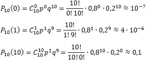
Задача. Вероятность выпуска бракованного изделия на станке равна 0,2. Определить вероятность того, что в партии из десяти выпущенных на данном станке деталей ровно k будут без брака. Решить задачу для k = 0, 1, 10.

По условию, нас интересует событие A выпуска изделий без брака, которое случается каждый раз с вероятностью p = 1 − 0,2 = 0,8. Нужно определить вероятность того, что это событие произойдет k раз. Событию A противопоставляется событие «не A», т.е. выпуск бракованного изделия.

Таким образом, имеем: n = 10; p = 0,8; q = 0,2.

Итак, находим вероятность того, что в партии все детали бракованные (k = 0), что только одна деталь без брака (k = 1), и что бракованных деталей нет вообще (k = 10):

Задача. Монету бросают 6 раз. Выпадение герба и решки равновероятно. Найти вероятность того, что:

герб выпадет три раза;

герб выпадет один раз;

герб выпадет не менее двух раз.

Итак, нас интересует событие A, когда выпадает герб. Вероятность этого события равна p = 0,5. Событию A противопоставляется событие «не A», когда выпадает решка, что случается с вероятностью q = 1 − 0,5 = 0,5. Нужно определить вероятность того, что герб выпадет k раз.

Таким образом, имеем: n = 6; p = 0,5; q = 0,5.

Определим вероятность того, что герб выпал три раза, т.е. k = 3:

Теперь определим вероятность того, что герб выпал только один раз, т.е. k = 1:

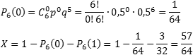
Осталось определить, с какой вероятностью герб выпадет не менее двух раз. Основная загвоздка — во фразе «не менее». Получается, что нас устроит любое k, кроме 0 и 1, т.е. надо найти значение суммы X = P₆(2) + P₆(3) + … + P₆(6).

Заметим, что эта сумма также равна (1 − P₆(0) − P₆(1)), т.е. достаточно из всех возможных вариантов «вырезать» те, когда герб выпал 1 раз (k = 1) или не выпал вообще (k = 0). Поскольку P₆(1) нам уже известно, осталось найти P₆(0):

Задача. Вероятность того, что телевизор имеет скрытые дефекты, равна 0,2. На склад поступило 20 телевизоров. Какое событие вероятнее: что в этой партии имеется два телевизора со скрытыми дефектами или три?

Интересующее событие A — наличие скрытого дефекта. Всего телевизоров n = 20, вероятность скрытого дефекта p = 0,2. Соответственно, вероятность получить телевизор без скрытого дефекта равна q = 1 − 0,2 = 0,8.

Получаем стартовые условия для схемы Бернулли: n = 20; p = 0,2; q = 0,8.

Найдем вероятность получить два «дефектных» телевизора (k = 2) и три (k = 3):

[begin{array}{l}{P_{20}}left( 2 right) = C_{20}^2{p^2}{q^{18}} = frac{{20!}}{{2!18!}} cdot {0,2^2} cdot {0,8^{18}} approx 0,137\{P_{20}}left( 3 right) = C_{20}^3{p^3}{q^{17}} = frac{{20!}}{{3!17!}} cdot {0,2^3} cdot {0,8^{17}} approx 0,41end{array}]

Очевидно, P₂₀(3) > P₂₀(2), т.е. вероятность получить три телевизора со скрытыми дефектами больше вероятности получить только два таких телевизора. Причем, разница неслабая.

Небольшое замечание по поводу факториалов. Многие испытывают смутное ощущение дискомфорта, когда видят запись «0!» (читается «ноль факториал»). Так вот, 0! = 1 по определению.

P. S. А самая большая вероятность в последней задаче — это получить четыре телевизора со скрытыми дефектами. Подсчитайте сами — и убедитесь.

Смотрите также:

Локальная теорема Муавра — Лапласа
Формула полной вероятности
Тест к уроку «Сложение и вычитание дробей» (легкий)
Сводный тест по задачам B12 (2 вариант)
Как решать задачи про летающие камни?
Задача C1: тригонометрические уравнения и формула двойного угла

Источник

Повторные независимые испытания.
Схема и формула Бернулли

Определение повторных независимых испытаний. Формулы Бернулли для вычисления вероятности и наивероятнейшего числа. Асимптотические формулы для формулы Бернулли (локальная и интегральная, теоремы Лапласа). Использование интегральной теоремы. Формула Пуассона, для маловероятных случайных событий.

Повторные независимые испытания

На практике приходится сталкиваться с такими задачами, которые можно представить в виде многократно повторяющихся испытаний, в результате каждого из которых может появиться или не появиться событие . При этом интерес представляет исход не каждого «отдельного испытания, а общее количество появлений события в результате определенного количества испытаний. В подобных задачах нужно уметь определять вероятность любого числа появлений события в результате испытаний. Рассмотрим случай, когда испытания являются независимыми и вероятность появления события в каждом испытании постоянна. Такие испытания называются повторными независимыми.

Примером независимых испытаний может служить проверка на годность изделий, взятых по одному из ряда партий. Если в этих партиях процент брака одинаков, то вероятность того, что отобранное изделие будет бракованным, в каждом случае является постоянным числом.

Формула Бернулли

Воспользуемся понятием сложного события, под которым подразумевается совмещение нескольких элементарных событий, состоящих в появлении или непоявлении события в –м испытании. Пусть проводится независимых испытаний, в каждом из которых событие может либо появиться с вероятностью , либо не появиться с вероятностью q=1-p . Рассмотрим событие B_m , состоящее в том, что событие в этих испытаниях наступит ровно раз и, следовательно, не наступит ровно (n-m) раз. Обозначим $A_i~(i=1,2,ldots,{n})$ появление события , a $overline{A}_i$ — непоявление события в –м испытании. В силу постоянства условий испытания имеем

$begin{gathered}P{A_1}=P{A_2}=cdots=P{A_n}=p,\P{overline{A}_1}=P{overline{A}_2}=cdots=P{overline{A}_n}=1-p=qend{gathered}$

Событие может появиться раз в разных последовательностях или комбинациях, чередуясь с противоположным событием overline{A} . Число возможных комбинаций такого рода равно числу сочетаний из элементов по , т. е. C_n^m . Следовательно, событие B_m можно представить в виде суммы сложных несовместных между собой событий, причем число слагаемых равно C_n^m :

$B_m=A_1A_2cdots{A_m}overline{A}_{m+1}cdotsoverline{A}_n+cdots+overline{A}_1overline{A}_2cdotsoverline{A}_{n-m}A_{n-m+1}cdots{A_n},$

(3.1)

где в каждое произведение событие входит раз, а overline{A} — (n-m) раз.

Вероятность каждого сложного события, входящего в формулу (3.1), по теореме умножения вероятностей для независимых событий равна $p^{m}q^{n-m}$ . Так как общее количество таких событий равно C_n^m , то, используя теорему сложения вероятностей для несовместных событий, получаем вероятность события B_m (обозначим ее $P_{m,n}$ )

$P_{m,n}=C_n^mp^{m}q^{n-m}quad text{or}quad P_{m,n}=frac{n!}{m!(n-m)!}p^{m}q^{n-m}.$

(3.2)

Формулу (3.2) называют формулой Бернулли, а повторяющиеся испытания, удовлетворяющие условию независимости и постоянства вероятностей появления в каждом из них события , называют испытаниями Бернулли, или схемой Бернулли.

Пример 1. Вероятность выхода за границы поля допуска при обработке деталей на токарном станке равна 0,07. Определить вероятность того, что из пяти наудачу отобранных в течение смены деталей у одной размеры диаметра не соответствуют заданному допуску.

Решение. Условие задачи удовлетворяет требования схемы Бернулли. Поэтому, полагая n=5,,m=1,,p=0,!07 , по формуле (3.2) получаем

$P_{1,5}=C_5^1(0,!07)^{1}(0,!93)^{5-1}approx0,!262.$

Пример 2. Наблюдениями установлено, что в некоторой местности в сентябре бывает 12 дождливых дней. Какова вероятность того, что из случайно взятых в этом месяце 8 дней 3 дня окажутся дождливыми?

Решение.

$P_{3;8}=C_8^3{left(frac{12}{30}right)!}^3{left(1-frac{12}{30}right)!}^{8-3}=frac{8!}{3!(8-3)!}{left(frac{2}{5}right)!}^3{left(frac{3}{5}right)!}^5=56cdotfrac{8}{125}cdotfrac{243}{3125}=frac{108,864}{390,625}approx0,!2787.$

Наивероятнейшее число появлений события

Наивероятнейшим числом появления события в независимых испытаниях называется такое число m_0 , для которого вероятность, соответствующая этому числу, превышает или, по крайней мере, не меньше вероятности каждого из остальных возможных чисел появления события . Для определения наивероятнейшего числа не обязательно вычислять вероятности возможных чисел появлений события, достаточно знать число испытаний и вероятность появления события в отдельном испытании. Обозначим $P_{m_0,n}$ вероятность, соответствующую наивероятнейшему числу m_0 . Используя формулу (3.2), записываем

$P_{m_0,n}=C_n^{m_0}p^{m_0}q^{n-m_0}=frac{n!}{m_0!(n-m_0)!}p^{m_0}q^{n-m_0}.$

(3.3)

Согласно определению наивероятнейшего числа, вероятности наступления события соответственно m_0+1 и m_0-1 раз должны, по крайней мере, не превышать вероятность $P_{m_0,n}$ , т. е.

$P_{m_0,n}geqslant{P_{m_0+1,n}};quad P_{m_0,n}geqslant{P_{m_0-1,n}}$

Подставляя в неравенства значение $P_{m_0,n}$ и выражения вероятностей $P_{m_0+1,n}$ и $P_{m_0-1,n}$ , получаем

$begin{gathered}frac{n!}{m_0!(n-m_0)!}p^{m_0}q^{n-m_0}geqslantfrac{n!}{(m_0+1)!(n-m_0-1)!}p^{m_0+1}q^{n-m_0-1}\\frac{n!}{m_0!(n-m_0)!}p^{m_0}q^{n-m_0}geqslantfrac{n!}{(m_0-1)!(n-m_0+1)!}p^{m_0-1}q^{n-m_0+1}end{gathered}$

Решая эти неравенства относительно m_0 , получаем

$m_0geqslant{np-q},quad m_0leqslant{np+p}$

Объединяя последние неравенства, получаем двойное неравенство, которое используют для определения наивероятнейшего числа:

$np-qleqslant{m_0}leqslant{np+p}.$

(3.4)

Так как длина интервала, определяемого неравенством (3.4), равна единице, т. е.

(np+p)-(np-q)=p+q=1,

и событие может произойти в испытаниях только целое число раз, то следует иметь в виду, что:

1) если np-q — целое число, то существуют два значения наивероятнейшего числа, а именно: m_0=np-q и m'_0=np-q+1=np+p ;

2) если np-q — дробное число, то существует одно наивероятнейшее число, а именно: единственное целое, заключенное между дробными числами, полученными из неравенства (3.4);

3) если — целое число, то существует одно наивероятнейшее число, а именно: m_0=np .

При больших значениях пользоваться формулой (3.3) для расчета вероятности, соответствующей наивероятнейшему числу, неудобно. Если в равенство (3.3) подставить формулу Стирлинга

$n!approx{n^ne^{-n}sqrt{2pi{n}}},$

справедливую для достаточно больших , и принять наивероятнейшее число m_0=np , то получим формулу для приближенного вычисления вероятности, соответствующей наивероятнейшему числу:

$P_{m_0,n}approxfrac{n^ne^{-n}sqrt{2pi{n}},p^{np}q^{nq}}{(np)^{np}e^{-np}sqrt{2pi{np}},(nq)^{nq}e^{-nq}sqrt{2pi{nq}}}=frac{1}{sqrt{2pi{npq}}}=frac{1}{sqrt{2pi}sqrt{npq}}.$

(3.5)

Пример 2. Известно, что $frac{1}{15}$ часть продукции, поставляемой заводом на торговую базу, не удовлетворяет всем требованиям стандарта. На базу была завезена партия изделий в количестве 250 шт. Найти наивероятнейшее число изделий, удовлетворяющих требованиям стандарта, и вычислить вероятность того, что в этой партии окажется наивероятнейшее число изделий.

Решение. По условию $n=250,,q=frac{1}{15},,p=1-frac{1}{15}=frac{14}{15}$ . Согласно неравенству (3.4) имеем

$250cdotfrac{14}{15}-frac{1}{15}leqslant{m_0}leqslant250cdotfrac{14}{15}+frac{14}{15}$

откуда $233,!26leqslant{m_0}leqslant234,!26$ . Следовательно, наивероятнейшее число изделий, удовлетворяющих требованиям стандарта, в партии из 250 шт. равно 234. Подставляя данные в формулу (3.5), вычисляем вероятность наличия в партии наивероятнейшего числа изделий:

$P_{234,250}approxfrac{1}{sqrt{2picdot250cdotfrac{14}{15}cdotfrac{1}{15}}}approx0,!101$

Локальная теорема Лапласа

Пользоваться формулой Бернулли при больших значениях очень трудно. Например, если n=50,,m=30,,p=0,!1 , то для отыскания вероятности $P_{30,50}$ надо вычислить значение выражения

$P_{30,50}=frac{50!}{30!cdot20!}cdot(0,!1)^{30}cdot(0,!9)^{20}$

Естественно, возникает вопрос: нельзя ли вычислить интересующую вероятность, не используя формулу Бернулли? Оказывается, можно. Локальная теорема Лапласа дает асимптотическую формулу, которая позволяет приближенно найти вероятность появления событий ровно раз в испытаниях, если число испытаний достаточно велико.

Теорема 3.1. Если вероятность появления события в каждом испытании постоянна и отлична от нуля и единицы, то вероятность $P_{m,n}$ того, что событие появится в испытаниях ровно раз, приближенно равна (тем точнее, чем больше ) значению функции

$y=frac{1}{sqrt{npq}}frac{e^{-x^2/2}}{sqrt{2pi}}=frac{varphi(x)}{sqrt{npq}}$ при $x=frac{m-np}{sqrt{npq}}$ .

Существуют таблицы, которые содержат значения функции $varphi(x)=frac{1}{sqrt{2pi}},e^{-x^{2}/2}$ , соответствующие положительным значениям аргумента . Для отрицательных значений аргумента используют те же таблицы, так как функция четна, т. е. varphi(-x)=varphi(x) .

Итак, приближенно вероятность того, что событие появится в испытаниях ровно раз,

$P_{m,n}approxfrac{1}{sqrt{npq}},varphi(x),$ где $x=frac{m-np}{sqrt{npq}}$ .

Пример 3. Найти вероятность того, что событие наступит ровно 80 раз в 400 испытаниях, если вероятность появления события в каждом испытании равна 0,2.

Решение. По условию n=400,,m=80,,p=0,!2,,q=0,!8 . Воспользуемся асимптотической, формулой Лапласа:

$P_{80,400}approxfrac{1}{sqrt{400cdot0,!2cdot0,!8}},varphi(x)=frac{1}{8},varphi(x).$

Вычислим определяемое данными задачи значение :

$x=frac{m-np}{sqrt{npq}}=frac{80-400cdot0,!2}{8}=0.$

По таблице прил, 1 находим varphi(0)=0,!3989 . Искомая вероятность

$P_{80,100}=frac{1}{8}cdot0,!3989=0,!04986.$

Формула Бернулли приводит примерно к такому же результату (выкладки ввиду их громоздкости опущены):

$P_{80,100}=0,!0498.$

Интегральная теорема Лапласа

Предположим, что проводится независимых испытаний, в каждом из которых вероятность появления события постоянна и равна . Необходимо вычислить вероятность $P_{(m_1,m_2),n}$ того, что событие появится в испытаниях не менее m_1 и не более m_2 раз (для краткости будем говорить «от m_1 до m_2 раз»). Это можно сделать с помощью интегральной теоремы Лапласа.

Теорема 3.2. Если вероятность наступления события в каждом испытании постоянна и отлична от нуля и единицы, то приближенно вероятность $P_{(m_1,m_2),n}$ того, что событие появится в испытаниях от m_1 до m_2 раз,

$P_{(m_1,m_2),n}approxfrac{1}{sqrt{2pi}}intlimits_{x'}^{x''}e^{-x^2/2},dx,$ где $x'=frac{m_1-np}{sqrt{npq}};~x''=frac{m_2-np}{sqrt{npq}}$ .

При решении задач, требующих применения интегральной теоремы Лапласа, пользуются специальными таблицами, так как неопределенный интеграл $int{e^{-x^2/2},dx}$ не выражается через элементарные функции. Таблица для интеграла $Phi(x)=frac{1}{sqrt{2pi}}intlimits_{0}^{x}e^{-z^2/2},dz$ приведена в прил. 2, где даны значения функции Phi(x) для положительных значений , для x<0 используют ту же таблицу (функция Phi(x) нечетна, т. е. Phi(-x)=-Phi(x) ). Таблица содержит значения функции Phi(x) лишь для xin[0;5] ; для x>5 можно принять Phi(x)=0,!5 .

Итак, приближенно вероятность того, что событие появится в независимых испытаниях от m_1 до m_2 раз,

$P_{(m_1,m_2),n}approxPhi(x'')-Phi(x'),$ где $x'=frac{m_1-np}{sqrt{npq}};~x''=frac{m_2-np}{sqrt{npq}}$ .

Пример 4. Вероятность того, что деталь изготовлена с нарушениями стандартов, p=0,!2 . Найти вероятность того, что среди 400 случайно отобранных деталей нестандартных окажется от 70 до 100 деталей.

Решение. По условию p=0,!2,,q=0,!8,,n=400,,m_1=70,,m_2=100 . Воспользуемся интегральной теоремой Лапласа:

$P_{(70,100),400}approxPhi(x'')-Phi(x').$

Вычислим пределы интегрирования:

нижний

$x'=frac{m_1-np}{sqrt{npq}}=frac{70-400cdot0,!2}{sqrt{400cdot0,!2cdot0,!8}}=-1,!25,$

верхний

$x''=frac{m_2-np}{sqrt{npq}}=frac{100-400cdot0,!2}{sqrt{400cdot0,!2cdot0,!8}}=2,!5,$

Таким образом

$P_{(70,100),400}approxPhi(2,!5)-Phi(-1,!25)=Phi(2,!5)+Phi(1,!25).$

По таблице прил. 2 находим

Phi(2,!5)=0,!4938;~~~~~Phi(1,!25)=0,!3944.

Искомая вероятность

$P_{(70,100),400}=0,!4938+0,!3944=0,!8882.$

Применение интегральной теоремы Лапласа

Если число (число появлений события при независимых испытаниях) будет изменяться от m_1 до m_2 , то дробь $frac{m-np}{sqrt{npq}}$ будет изменяться от $frac{m_1-np}{sqrt{npq}}=x'$ до $frac{m_2-np}{sqrt{npq}}=x''$ . Следовательно, интегральную теорему Лапласа можно записать и так:

$Pleft{x'leqslantfrac{m-np}{sqrt{npq}}leqslant{x''}right}=frac{1}{sqrt{2pi}}intlimits_{x'}^{x''}e^{-x^2/2},dx.$

(3.6)

Поставим задачу найти вероятность того, что отклонение относительной частоты $frac{m}{n}$ от постоянной вероятности по абсолютной величине не превышает заданного числа varepsilon>0 . Другими словами, найдем вероятность осуществления неравенства $left|frac{m}{n}-pright|leqslantvarepsilon$ , что то же самое, $-varepsilonleqslantfrac{m}{n}-pleqslantvarepsilon$ . Эту вероятность будем обозначать так: $Pleft{left|frac{m}{n}-pright|leqslantvarepsilonright}$ . С учетом формулы (3.6) для данной вероятности получаем

$Pleft{left|frac{m}{n}-pright|leqslantvarepsilonright}approx2Phileft(varepsilon,sqrt{frac{n}{pq}}right).$

(3.7)

Пример 5. Вероятность того, что деталь нестандартна, p=0,!1 . Найти вероятность того, что среди случайно отобранных 400 деталей относительная частота появления нестандартных деталей отклонится от вероятности p=0,!1 по абсолютной величине не более чем на 0,03.

Решение. По условию n=400,,p=0,!1,,q=0,!9,,varepsilon=0,!03 . Требуется найти вероятность $Pleft{left|frac{m}{400}-0,!1right|leqslant0,!03right}$ . Используя формулу (3.7), получаем

$Pleft{left|frac{m}{400}-0,!1right|leqslant0,!03right}approx2Phileft(0,!03sqrt{frac{400}{0,!1cdot0,!9}}right)=2Phi(2)$

По таблице прил. 2 находим Phi(2)=0,!4772 , следовательно, 2Phi(2)=0,!9544 . Итак, искомая вероятность приближенно равна 0,9544. Смысл полученного результата таков: если взять достаточно большое число проб по 400 деталей в каждой, то примерно в 95,44% этих проб отклонение относительной частоты от постоянной вероятности p=0,!1 по абсолютной величине не превысит 0,03.

Формула Пуассона для маловероятных событий

Если вероятность наступления события в отдельном испытании близка к нулю, то даже при большом числе испытаний , но при небольшом значении произведения получаемые по формуле Лапласа значения вероятностей $P_{m,n}$ оказываются недостаточно точными и возникает потребность в другой приближенной формуле.

Теорема 3.3. Если вероятность наступления события в каждом испытании постоянна, но мала, число независимых испытаний достаточно велико, но значение произведения np=lambda остается небольшим (не больше десяти), то вероятность того, что в этих испытаниях событие наступит раз,

$P_{m,n}approxfrac{lambda^m}{m!},e^{-lambda}.$

Для упрощения расчетов с применением формулы Пуассона составлена таблица значений функции Пуассона $frac{lambda^m}{m!},e^{-lambda}$ (см. прил. 3).

Пример 6. Пусть вероятность изготовления нестандартной детали равна 0,004. Найти вероятность того, что среди 1000 деталей окажется 5 нестандартных.

Решение. Здесь n=1000,p=0,004,~lambda=np=1000cdot0,!004=4 . Все три числа удовлетворяют требованиям теоремы 3.3, поэтому для нахождения вероятности искомого события $P_{5,1000}$ применяем формулу Пуассона. По таблице значений функции Пуассона (прил. 3) при lambda=4;m=5 получаем $P_{5,1000}approx0,!1563$ .

Найдем вероятность того же события по формуле Лапласа. Для этого сначала вычисляем значение , соответствующее m=5 :

$x=frac{5-1000cdot0,!004}{sqrt{1000cdot0,!004cdot0,!996}}approxfrac{1}{1,!996}approx0,!501.$

Поэтому согласно формуле Лапласа искомая вероятность

$P_{5,1000}approxfrac{varphi(0,!501)}{1,!996}approxfrac{0,!3519}{1,!996}approx0,!1763$

а согласно формуле Бернулли точное ее значение

$P_{5,1000}=C_{1000}^{5}cdot0,!004^5cdot0,!996^{995}approx0,!1552.$

Таким образом, относительная ошибка вычисления вероятностей $P_{5,1000}$ по приближенной формуле Лапласа составляет

$frac{0,!1763-0,!1552}{0,!1552}approx0,!196$ , или 13,!6%

а по формуле Пуассона —

$frac{0,!1563-0,!1552}{0,!1552}approx0,!007$ , или 0,!7%

т.е. во много раз меньше.

Математический форум (помощь с решением задач, обсуждение вопросов по математике).

Кнопка "Поделиться"

Если заметили ошибку, опечатку или есть предложения, напишите в комментариях.

Источник

Число Бернулли

B₀ = 1

$B_1=-frac12$

$B_2=frac16$

B₃ = 0

$B_4=-frac1{30}$

B₅ = 0

$B_6=frac1{42}$

B₇ = 0

$B_8=-frac1{30}$

B₉ = 0

$B_{10}=frac5{66}$

B₁₁ = 0

$B_{12}=-frac{691}{2730}$

B₁₃ = 0

$B_{14}=frac76$

B₁₅ = 0

$B_{16}=-7frac{47}{510}$

Числа Бернулли — последовательность рациональных чисел B₀,B₁,B₂,… найденная Я. Бернулли в связи с вычислением суммы одинаковых степеней натуральных чисел:

$sum_{n=1}^{N-1} n^k=frac1{k+1}sum_{s=0}^kC^s_{k+1}B_s N^{k+1-s}$

Содержание

1 Формула для чисел Бернулли
2 Свойства
3 Литература
4 Ссылки

Формула для чисел Бернулли

Для чисел Бернулли существует следующая реккурентная формула: $B_n=frac{-1}{n+1}sum_{k=1}^{n}C_{n+1}^{k+1}B_{n-k},quad ninmathbb{N}$

Свойства

Все числа Бернулли с нечетными номерами, кроме B₁, равны нулю, знаки B_2n чередуются.
Числа Бернулли являются значениями при x = 0 многочленов Бернулли: B_n = B_n(0).

Коэффициентами разложения некоторых элементарных функций в степенные ряды часто служат числа Бернулли. Например:

Экспоненциальная производящая функция для чисел Бернулли:

$frac x{e^x-1}=sum_{n=0}^inftyfrac{B_n}{n!}x^n, |x|&lt; 2pi$

$B_{2k}=2(-1)^{k+1}frac {zeta(2k); (2k)!} {(2pi)^{2k}}.$

Из чего следует

B_n = − nζ(1 − n) для всех n.

$intlimits_0^infty frac{x^{2n-1}dx}{e^{2pi x}-1}=frac1{4n}|B_{2n}|, n=1,2,...$

Литература

Абрамович В. Числа Бернулли, Квант, № 6, 1974;

Ссылки

Генератор Чисел Бернули

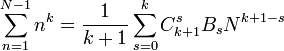
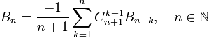
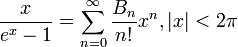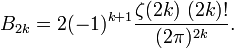
Wikimedia Foundation.
2010.

Полезное

Смотреть что такое «Число Бернулли» в других словарях:

число Бернулли — Bernulio skaičius statusas T sritis fizika atitikmenys: angl. Bernoulli’s number vok. Bernoulli Zahl, f rus. бернуллиево число, n; число Бернулли, n pranc. nombre bernoullien, m … Fizikos terminų žodynas
Бернулли уравнение (дифференциальное) — Бернулли уравнение, дифференциальное уравнение 1 го порядка вида: dy/dx + Py = Qya, где Р, Q ‒ заданные непрерывные функции от x; a ‒ постоянное число. Введением новой функции z = y a+1 Б. у. сводится к линейному дифференциальному уравнению… … Большая советская энциклопедия
БЕРНУЛЛИ ИСПЫТАНИЯ — независимые испытания с двумя исходами каждое ( успехом и неудачей ) и такие, что вероятности исходов не изменяются от испытания к испытанию. Б. и. служат одной из основных схем, рассматриваемых в теории вероятностей. Пусть р вероятность успеха и … Математическая энциклопедия
БЕРНУЛЛИ ТЕОРЕМА — исторически первая форма больших чисел закона. Б. т. приведена в четвертой части книги Я. Бернулли (J. Bernoulli) Ars conjeсtandi ( Искусство предположений ). Эту часть можно считать первым серьезным трудом по теории вероятностей. Книга издана в… … Математическая энциклопедия
Бернулли уравнение — I Бернулли уравнение дифференциальное уравнение 1 го порядка вида: dy/dx + Py = Qyα, где Р, Q заданные непрерывные функции от x; α постоянное число. Введением новой функции z = y α+1 Б. у. сводится к линейному… … Большая советская энциклопедия
БЕРНУЛЛИ БЛУЖДАНИЕ — случайное блуждание, порождаемое Бернулли испытаниями. На примере Б. б. можно пояснить нек рые основные черты более общих случайных блужданий. В частности, уже в этой простейшей схеме проявляются свойства случайности , парадоксальные с точки… … Математическая энциклопедия
Число E — e математическая константа, основание натурального логарифма, иррациональное и трансцендентное число. Иногда число e называют числом Эйлера (не путать с т. н. числами Эйлера I рода) или числом Непера. Обозначается строчной латинской буквой «e».… … Википедия
Число e — e математическая константа, основание натурального логарифма, иррациональное и трансцендентное число. Иногда число e называют числом Эйлера (не путать с т. н. числами Эйлера I рода) или числом Непера. Обозначается строчной латинской буквой «e».… … Википедия
Число Эйлера — e математическая константа, основание натурального логарифма, иррациональное и трансцендентное число. Иногда число e называют числом Эйлера (не путать с т. н. числами Эйлера I рода) или числом Непера. Обозначается строчной латинской буквой «e».… … Википедия
Число е — e математическая константа, основание натурального логарифма, иррациональное и трансцендентное число. Иногда число e называют числом Эйлера (не путать с т. н. числами Эйлера I рода) или числом Непера. Обозначается строчной латинской буквой «e».… … Википедия

Источник

Notation[edit]

History[edit]

Early history[edit]

Reconstruction of «Summae Potestatum»[edit]

Definitions[edit]

Recursive definition[edit]

Explicit definition[edit]

Generating function[edit]

Bernoulli numbers and the Riemann zeta function[edit]

Efficient computation of Bernoulli numbers[edit]

Applications of the Bernoulli numbers[edit]

Asymptotic analysis[edit]

Sum of powers[edit]

Taylor series[edit]

Laurent series[edit]

Use in topology[edit]

Connections with combinatorial numbers[edit]

Connection with Worpitzky numbers[edit]

Connection with Stirling numbers of the second kind[edit]

Connection with Stirling numbers of the first kind[edit]

Connection with Pascal’s triangle[edit]

Connection with Eulerian numbers[edit]

A binary tree representation[edit]

Integral representation and continuation[edit]

The relation to the Euler numbers and π[edit]

An algorithmic view: the Seidel triangle[edit]

A combinatorial view: alternating permutations[edit]

[edit]

Arithmetical properties of the Bernoulli numbers[edit]

The Kummer theorems[edit]

p-adic continuity[edit]

Ramanujan’s congruences[edit]

Von Staudt–Clausen theorem[edit]

Why do the odd Bernoulli numbers vanish?[edit]

A restatement of the Riemann hypothesis[edit]

Generalized Bernoulli numbers[edit]

Eisenstein–Kronecker number[edit]

Appendix[edit]

Assorted identities[edit]

See also[edit]

Notes[edit]

References[edit]

External links[edit]

Схема повторных независимых испытаний. Формула Бернулли

Краткая теория

Схема Бернулли

Теорема Бернулли

Примеры решения задач

Пример 1

Пример 2

Пример 3

Задачи контрольных и самостоятельных работ

Схема Бернулли. Примеры решения задач

Повторные независимые испытания.Схема и формула Бернулли

Повторные независимые испытания

Формула Бернулли

Наивероятнейшее число появлений события

Локальная теорема Лапласа

Интегральная теорема Лапласа

Применение интегральной теоремы Лапласа

Формула Пуассона для маловероятных событий

Число Бернулли

Содержание

Формула для чисел Бернулли

Свойства

Литература

Ссылки

Полезное

Смотреть что такое «Число Бернулли» в других словарях:

Не пропустите также:

Схема повторных независимых испытаний.
Формула Бернулли

Повторные независимые испытания.
Схема и формула Бернулли