Базис френе как найти

Содержание

Касательная, нормальная плоскость, соприкасающаяся плоскость, бинормаль, главная нормаль, репер Френе

Краткие теоретические сведения

Кривая в пространстве

Рассмотрим в пространстве гладкую кривую $gamma$.

Векторное уравнение $gamma:, vec{r}=vec{r}(t)$.
Параметрическое уравнение $gamma:,, x=x(t),, y=y(t),, z=z(t)$.

Пусть точка $M$ принадлежит данной кривой и отвечает значению параметра $t=t_0$. Тогда радиус-вектор и координаты данной точки равны:

begin{equation*}
vec{r_0}=vec{r}(t_0), quad x_0=x(t_0),, y_0=y(t_0), , z_0=z(t_0).
end{equation*}

Пусть в точке $M$ $ vec{r’}(t_0)neqvec{0}$, то есть $M$ не является особой точкой.

Касательная к кривой

Касательная к кривой, проведенная в точке $M$, имеет направляющий вектор коллинеарный вектору $vec{r’}(t_0)$.

Пусть $vec{R}$ — радиус-вектор произвольной точки касательной, тогда уравнение этой касательной имеет вид

begin{equation*}
vec{R}=vec{r}(t_0)+lambdavec{r’}(t_0).
end{equation*}

Здесь $lambdain(-infty,+infty)$ — параметр, определяющий положение точки на касательной (то есть разным значениям $lambda$ будут соответствовать разные значения $vec{R}$).

Если $vec{R}={X,Y,Z}$, $M = (x(t_0), y(t_0), z(t_0))$, то можно записать уравнение касательной в каноническом виде:

begin{equation*}
frac{X-x(t_0)}{x'(t_0)}=frac{Y-y(t_0)}{y'(t_0)}=frac{Z-z(t_0)}{z'(t_0)}.
end{equation*}

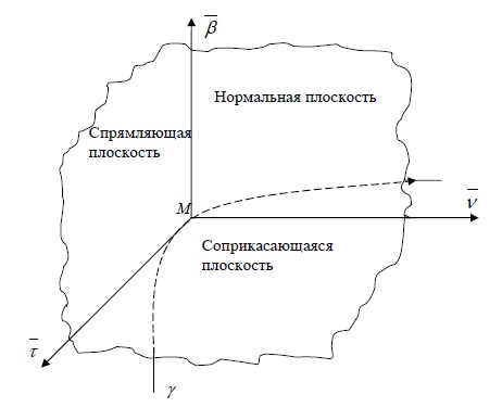
Нормальная плоскость

Плоскость, проходящую через данную точку $M$ кривой $gamma$ перпендикулярно касательной в этой точке, называют нормальной плоскостью.

Пусть $vec{R}$ — радиус-вектор произвольной точки нормальной плоскости, тогда ее уравнение можно записать в векторном виде через скалярное произведение векторов $vec{R}-vec{r}(t_0)$ и $vec{r’}(t_0)$:

begin{equation*}
(vec{R}-vec{r}(t_0))cdotvec{r’}(t_0)=0.
end{equation*}

Если расписать покоординатно, то получим следующее уравнение:

begin{equation*}
x'(t_0)cdot(X-x(t_0))+y'(t_0)cdot(Y-y(t_0))+z'(t_0)cdot(Z-z(t_0))=0.
end{equation*}

Соприкасающаяся плоскость

Плоскость, проходящую через заданную точку $M$ кривой $gamma$ параллельно векторам $vec{r’}(t_0)$, $vec{r»}(t_0)$, когда они неколлинеарны, называют соприкасающейся плоскостью кривой.

Если $vec{R}$ — радиус-вектор произвольной точки соприкасающейся плоскости, то ее уравнение можно записать через смешанной произведение трех компланарных векторов $vec{R}-vec{r}(t_0)$, $vec{r’}(t_0)$, $vec{r»}(t_0)$:

begin{equation*}
(vec{R}-vec{r}(t_0), vec{r’}(t_0), vec{r»}(t_0))=0.
end{equation*}

Зная координаты точки и векторов, определяющих плоскость, запишем смешанное произведение через определитель. Получим следующее уравнение соприкасающейся плоскости:

begin{equation*}
left|
begin{array}{ccc}
X-x(t_0) & Y-y(t_0) & Z-z(t_0) \
x'(t_0) & y'(t_0) & z'(t_0)\
x»(t_0) & y»(t_0) & z»(t_0) \
end{array}
right|=0
end{equation*}

Плоская кривая лежит в своей соприкасающейся плоскости.

Бинормаль и главная нормаль

Прямая, проходящая через точку $M$ кривой $gamma$ перпендикулярно касательной к кривой в этой точке, называется нормалью.

Таких кривых можно провести бесконечно много, все они образуют нормальную плоскость. Мы выделим среди нормалей две — бинормаль и главную нормаль.

Нормаль, перпендикулярную соприкасающейся плоскости, называют бинормалью.

Нормаль, лежащую в соприкасающейся плоскости, называют главной нормалью.

Из определения бинормали (перпендикулярна касательной и перпендикулярна соприкасающейся плоскости) следует, что в качестве ее направляющего вектора мы можем взять векторное произведение $ vec{r’}(t_0)timesvec{r»}(t_0)$, тогда ее уравнение можно записать в виде:

begin{equation*}
vec{R}=vec{r}(t_0)+lambda,vec{r’}(t_0)timesvec{r»}(t_0).
end{equation*}

Как и раньше, $vec{R}$ — радиус-вектор произвольной точки бинормали.
Каноническое уравнение прямой:

begin{equation*}
frac{X-x(t_0)}{left|
begin{array}{cc}
y'(t_0) & z'(t_0) \
y»(t_0) & z»(t_0) \
end{array}
right|
}=frac{Y-y(t_0)}{left|
begin{array}{cc}
z'(t_0) & x'(t_0) \
z»(t_0) & x»(t_0) \
end{array}
right|
}=frac{Z-z(t_0)}{left|
begin{array}{cc}
x'(t_0) & y'(t_0) \
x»(t_0) & y»(t_0) \
end{array}
right|
}.
end{equation*}

Из определения главной нормали (перпендикулярна касательной и перпендикулярна бинормали) следует, что в качестве ее направляющего вектора можно взять векторное произведение $vec{r’}(t_0) timesleft[vec{r’}(t_0),vec{r»}(t_0)right]$:

begin{equation*}
vec{R}=vec{r}(t_0)+lambda,vec{r’}(t_0) timesleft[vec{r’}(t_0),vec{r»}(t_0)right].
end{equation*}

Уравнение в каноническом виде распишите самостоятельно.

Спрямляющая плоскость

Плоскость, проходящую через заданную точку $M$ кривой $gamma$ перпендикулярно главной нормали, называют спрямляющей плоскостью.

Другое определение:
Плоскость, определяемую касательной к кривой и бинормалью в той же точке, называют спрямляющей плоскостью.

Второе определение позволяет записать уравнение спрямляющей плоскости через смешанное произведение трех компланарных векторов, определяющих эту плоскость $vec{R}-vec{r}(t_0)$, $vec{r’}(t_0)$, $vec{r’}(t_0)timesvec{r»}(t_0)$:
begin{equation*}
left(vec{R}-vec{r}(t_0),, vec{r’}(t_0),, vec{r’}(t_0)timesvec{r»}(t_0)right)=0.
end{equation*}
Зная координаты соответствующих векторов, можно легко записать это смешанное произведение через определитель, раскрыв который, вы получите общее уравнение спрямляющей плоскости.

Репер Френе

Орт (то есть единичный вектор) касательной обозначим:
$$ vec{tau}=frac{vec{r’}(t_0)}{|vec{r’}(t_0)|}. $$
Орт бинормали:
$$ vec{beta}=frac{vec{r’}(t_0)timesvec{r»}(t_0)}{|vec{r’}(t_0)timesvec{r»}(t_0)|}. $$
Орт главной нормали:
$$ vec{nu}=frac{vec{r’}(t_0) times[vec{r’}(t_0),,vec{r»}(t_0)]}{|vec{r’}(t_0) times [vec{r’}(t_0),,vec{r»}(t_0)]|}. $$

Правая тройка векторов $vec{tau}$, $vec{nu}$, $vec{beta}$ называется репером Френе.

Решение задач

Задача 1

Кривая $gamma$ задана параметрически:

$$
x=t,,, y=t^2,,, z=e^t.
$$

Точка $M$, принадлежащая кривой, соответствует значению параметра $t=0$.
Записать уравнения касательной, бинормали, главной нормали, нормальной плоскости, соприкасающейся плоскости и спрямляющей плоскости, проведенных к данной кривой в точке $M$. Записать векторы репера Френе.

Решение задачи 1

Задачу можно решать разными способами, точнее в разном порядке находить уравнения прямых и плоскостей.

Начнем с производных.

begin{gather*}
gamma: vec{r}(t)=left{ t,, t^2,, e^tright} ,, Rightarrow \
vec{r’}(t)=left{ 1,, 2t,, e^tright},\
vec{r»}(t)=left{ 0,, 2,, e^tright}.
end{gather*}
В точке $M(t_0=0)$:
begin{gather*}
vec{r}(t_0)={ 0,, 0,, 1},\
vec{r’}(t_0)={ 1,, 0,, 1},\
vec{r»}(t_0)={ 0,, 2,, 1}.
end{gather*}

Зная координаты точки $M(0,0,1)$ и направляющего вектора $ vec{r’}(t_0)={ 1,0,1 }$, можем записать уравнение касательной:

begin{equation*}
frac{X}{1}=frac{Y}{0}=frac{Z-1}{1}.
end{equation*}

Нормальная плоскость проходит через точку $M(0,0,1)$ перпендикулярно вектору $vec{r’}(t_0)={ 1,0,1 }$, поэтому ее общее уравнение имеет вид:

begin{equation*}
1cdot X+0cdot Y+1cdot (Z-1)=0,, Rightarrow ,, X+Z=1.
end{equation*}

Запишем теперь уравнение соприкасающейся плоскости, определяемой точкой $M(0,0,1)$ и векторами: $vec{r’}(t_0)={ 1,, 0,, 1}$, $vec{r»}(t_0)={ 0,, 2,, 1}$:

begin{equation*}
left|
begin{array}{ccc}
X-0 & Y-0 & Z-1 \
1 & 0 & 1\
0 & 2 & 1 \
end{array}
right|=0
end{equation*}
Раскрываем определитель, получаем уравнение:
begin{equation*}
-2X-Y+2Z-2=0
end{equation*}

Направление бинормали задается вектором $vec{r’}(t_0) times vec{r»}(t_0)$. Координаты этого вектора мы уже нашли, когда вычисляли миноры в определителе, задающем уравнение соприкасающейся плоскости.

$$
{ 1,, 0,, 1} times { 0,, 2,, 1}= left|
begin{array}{ccc}
vec{i} & vec{j} & vec{k} \
1 & 0 & 1\
0 & 2 & 1 \
end{array}
right|= {-2,, -1,, 2}.
$$

Уравнение бинормали:

begin{equation*}
frac{X}{-2}=frac{Y}{-1}=frac{Z-1}{2}.
end{equation*}

Направление главной нормали задается вектором $vec{r’}(t_0) times (vec{r’}(t_0)timesvec{r»}(t_0))$.

$$
{ 1,, 0,, 1} times {-2,, -1,, 2}= left|
begin{array}{ccc}
vec{i} & vec{j} & vec{k} \
1 & 0 & 1\
-2 & -1 & 2 \
end{array}
right|= {1,, -4,, -1} ,, Rightarrow ,,
frac{X}{1}=frac{Y}{-4}=frac{Z-1}{-1}.
$$

Спрямляющая плоскость перпендикулярна главной нормали, а значит, вектору ${1,, -4,, -1}$, поэтому можем сразу записать ее общее уравнение:

begin{equation*}
1cdot X-4cdot Y-1cdot (Z-1)=0,, Rightarrow ,, X-4Y-Z+1=0.
end{equation*}

Орт касательной: $vec{tau} =frac{1}{sqrt{2}}{1,,0,,1}$,
Орт главной нормали: $vec{nu} =frac{1}{sqrt{18}}{1,,-4,,-1}$,
Орт бинормали: $vec{beta }=frac{1}{3}{-2,,-1,,2}$.

Поскольку направляющий вектор главной нормали у нас был найден как векторное произведение направляющих векторов касательной и бинормали, тройка $vec{tau}$, $vec{nu}$, $vec{beta}$ не будет правой (по определению векторного произведения вектор $vec{tau}timesvec{beta}$ направлен так, что тройка векторов $vec{tau}$, $vec{beta}$, $vec{nu}=vec{tau}timesvec{beta}$ — правая). Изменим направление одного из векторов. Например, пусть

$$ vec{nu} =frac{1}{sqrt{18}}{-1,,4,,1}.$$

Теперь тройка $vec{tau}$, $vec{nu}$, $vec{beta}$ образует репер Френе для кривой $gamma$ в точке $M$.

Задача 2

Написать уравнение соприкасающейся плоскости к кривой
$$
x=t,,, y=frac{t^2}{2},,, z=frac{t^3}{3},
$$
проходящей через точку $N(0,0,9)$.

Решение задачи 2

Нетрудно заметить, что точка $N$ не принадлежит заданной кривой $gamma$. Следовательно соприкасающаяся плоскость проведена в какой-то точке $M(t=t_0)ingamma$, но при этом плоскость проходит через заданную точку $N(0,0,9)$.

Найдем значение параметра $t_0$.

Для этого запишем уравнение соприкасающейся плоскости, проведенной в произвольной точке $M(t=t_0)$. И учтем, что координаты $N$ должны удовлетворять полученному уравнению.

begin{align*}
gamma: vec{r}(t)&=left{ t,, frac{t^2}{2},, frac{t^3}{3}right} ,, Rightarrow \
vec{r’}(t)&=left{ 1,, t,, 3t^2right},\
vec{r»}(t)&=left{ 0,, 1,, 6tright}.
end{align*}
В точке $M(t=t_0)$:
begin{align*}
vec{r}(t_0)&=left{t_0,, frac{t_0^2}{2},, frac{t_0^3}{3}right} \
vec{r’}(t_0)&=left{1,, t_0,, 3t_0^2right},\
vec{r»}(t_0)&=left{0,, 1,, 6t_0right}.
end{align*}

Соприкасающаяся плоскость определяется векторами $vec{r’}(t_0)$, $vec{r»}(t_0)$, поэтому записываем определитель
begin{equation*}
left|
begin{array}{ccc}
X-t_0 & Y-t_0^2/2 & Z-t_0^3/3 \
&&\
1 & t_0 & t^2_0 \
&&\
0 & 1 & 2t_0
end{array}
right|=0 quad Rightarrow
end{equation*}

begin{equation*}
(X-t_0)cdot t_0^2 — (Y-t_0^2/2)cdot 2t_0 + (Z-t_0^3/3)=0.
end{equation*}
Подставляем вместо $X$, $Y$, $Z$ координаты точки $N$: $X=0$, $Y=0$, $Z=9$, упрощаем и получаем уравнение относительно $t_0$:
begin{equation*}
9-t_0^3/3=0 quad Rightarrow quad t_0=3.
end{equation*}
Подставив найденное $t_0$ в записанное ранее уравнение, запишем искомое уравнение соприкасающейся плоскости:
$$ 9X-6Y+Z-9=0. $$

Задача 3

Через точку $Pleft(-frac45,1,2right)$ провести плоскость, являющуюся спрямляющей для кривой:
$$
x=t^2,,, y=1+t,,, z=2t.
$$

Решение задачи 3

Как и в предыдущей задаче нам неизвестны координаты точки, в которой проведена спрямляющая плоскость к заданной кривой. Найдем их.

Спрямляющая плоскость определяется касательной и бинормалью, то есть векторами $vec{r’}(t_0)$ и $vec{r’}(t_0)timesvec{r»}(t_0)$.

В произвольной точке $M(t=t_0)$:
begin{align*}
vec{r}(t_0)&=left{t^2_0,, 1+t_0,, 2t_0right} \
vec{r’}(t_0)&=left{2t_0,, 1,, 2right},\
vec{r»}(t_0)&=left{2,, 0,, 0right}.
end{align*}
begin{equation*}
vec{r’}(t_0)timesvec{r»}(t_0)= left|
begin{array}{ccc}
vec{i} & vec{j} & vec{k} \
2t_0 & 1 & 2\
2 & 0 & 0
end{array}
right|= {0,, 4,, -2}
end{equation*}

Записываем уравнение спрямляющей плоскости:
begin{equation*}
left|
begin{array}{ccc}
X-t_0^2 & Y-1-t_0 & Z-2t_0 \
2t_0 & 1 & 2\
0 & 4 & -2
end{array}
right|= 0
end{equation*}

Раскрываем определитель. Подставляем в уравнение координаты точки $P$: $X=-4/5$, $Y=1$, $Z=2$. Упрощаем и получаем уравнение для нахождения $t_0$:
begin{equation*}
5t_0^2-8t_0-4=0 ,, Rightarrow ,, t_{01}=2,, t_{02}=-frac25.
end{equation*}

Уравнения соприкасающихся плоскостей к заданной кривой, проходящих через $P$, принимают вид:
begin{align*}
& 5X-4Y-8Z+24=0,\
& 25X+4Y+8Z=0.
end{align*}

Источник

В предыдущих параграфах были введены два единичных ортогональных вектора: вектор , направленный по касательной к кривой, и вектор главной нормали , который определён первой формулой Френе (1.9). Введём единичный вектор , ортогональный векторам и , как векторное произведение на

. (2.1)

Нормаль, которая определяется вектором , называется Бинормалью. Очевидно, что получена правая тройка ортогональных векторов. Этот подвижный базис (или репер), который сопровождает точку М при её движении по кривой, называется Подвижным, а также Естественным базисом или Репером Френе (Френе – французский геометр XIX века, который в 1847 году первым написал формулы для производных по длине дуги трёх базисных векторов , , ).

Плоскость, проходящая через вектора и , называется Соприкасающейся, через вектора и – Нормальной, а через вектора и – Спрямляющей. Эти три плоскости образуют так называемый Естественный трехгранник, или Трехгранник Френе (рис. 2.1).

Уравнение (1.9) определяет производную . Для того, чтобы получить производные от векторов и , обратимся к формуле (2.1). Дифференцируя по и используя формулу (1.9), имеем

Отсюда следует, что вектора и ортогональны. Кроме того, ортогонально (см п.3о в 1.2). Таким образом, направление вектора совпадает с направлением вектора главной нормали

. (2.2)

Это Вторая формула Френе, где коэффициент характеризует степень изменяемости вектора по длине дуги, то есть поворот соприкасающейся плоскости. Если , то кривая лежит в этой плоскости. Коэффициент называется кручением.

Теперь рассмотрим . Этот вектор ортогонален (по формуле (1.4)), поэтому в разложении по ортогональному базису , , ,

, (2.3)

Коэффициент .

Продифференцируем равенство

: .

В последнее соотношение подставим выражение из (2.3) и из (1.9). Получаем равенство , отсюда коэффициент .

Поскольку , получаем

. (2.4)

С другой стороны, по второй формуле Френе

Таким образом, С= , и

. (2.5)

Это Третья формула Френе.

По определению кривизна , но кручение может быть любого знака.

Для вычисления кручения используем вторую формулу Френе . Умножив скалярно на левую и правую части равенства, получим

С учётом равенства (см. формулу (2.4)), имеем

Где в круглых скобках записано смешанное произведение трёх векторов. Поскольку , а из первой формулы Френе следует, что , то

, (2.6)

Где в данном случае штрих означает дифференцирование по .

< Предыдущая		Следующая >

Источник

,
(6.9)

называется
длиной
дуги
пути
.

Теорема
6.4. Функция,
введённая формулой (6.9) в определении
6.13, на промежутке

непрерывна, монотонно возрастает, причём

и
.
Существует такая нигде непостоянная
параметризация

пути
,
что

Этим
условием параметризация

определена единственным образом.

Определение
6.5. Параметризация

спрямляемого
пути
,
построенная в теореме 6.4, называется
натуральной
параметризацией.

Имеет
место критерий натуральности
параметризация.

Теорема
6.5. Если

– гладкая параметризация спрямляемого
нигде непостоянного пути
,
то

является натуральной параметризацией
в том и только в том случае, если

и

,
то есть, вектор скорости

нормирован.

Следствие
из теоремы 6.5.
Если

– натуральная параметризация спрямляемого
нигде непостоянного пути
,
то вектор
ускорения

ортогонален вектору скорости
.

Д
о к а з а т е л ь с т в о. По доказанной
теореме в любой точке пути
,
то есть,
.
Дифференцируя последнее соотношение
по
,
получаем
.

Кривизна
пути в пространстве
.
Определим важную величину, характеризующую
скорость изменения направления
касательной в некоторой фиксированной
точке

пути
.
Предположим, что путь

является гладким и дважды непрерывно
дифференцируемым, то есть его параметризация
,
определённая координатными функциями,
является гладкой и дважды непрерывно
дифференцируемой вектор-функцией.
Направление касательной к пути в
фиксированной точке

задаётся вектором скорости, определяемым
по формуле (25):

В
точке
,
соответствующей на пути значению
параметра
,
вектор скорости равен

Угол между векторами
скорости пути

в точках

и
,
отнесённый к длине

дуги

пути, может служить мерой
искривлённости пути
на участке от точки

до точки
.
Эта мера называется
средней
кривизной

параметризованного пути

на дуге

и с учётом
формулы для косинуса угла между векторами

.
(7.1)

Формула (7.1) вполне
функциональна
– все входящие в неё величины легко
вычисляются.

Пример
7.1. Вычислить
среднюю кривизну окружности (9) радиуса

с центром в начале системы координат
на участке изменения параметра
.

Р
е ш е н и е. Из параметрических уравнений
окружности имеем:

,
,
,
,

,
.

Так
как
,
то по формуле (7.1) получаем

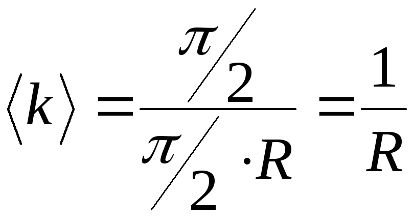Определение
7.1. Кривизной

параметризованного пути

в точке

(соответствующей значению параметра
)
называется предел при условии

отношения изменения

угла между векторами скорости

и

пути в начальной точке

и конечной точке

дуги

пути к её длине, то есть, предел при
условии

вдоль пути.

Итак,
для вычисления кривизны пути

с параметризацией
,
имеем следующую формулу:

.
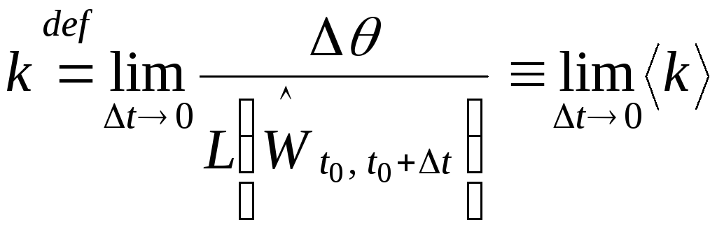(7.2)

Теорема
7.2. Пусть

– нигде непостоянный гладкий путь с
дважды непрерывно дифференцируемой
параметризацией
.
Тогда кривизна пути

в точке, соответствующей значению
параметра
,
определяется по формуле

.

(7.5)

Пример
7.2. Вычислить
кривизну окружности, имеющей радиус
,
в произвольной её точке.

Р
е ш е н и е. Воспользуемся формулой
(7.5). В координатах, связанных с плоскостью
окружности, её параметризация имеет
вид:

Находя
все величины из (7.5), получаем:

,
;

,
.

Откуда
имеем

Таким
образом, кривизна окружности равна
величине, обратной к её радиусу.

Трёхгранник
Френе. В
общем случае произвольной параметризации
можно построить ортонормированный
базис соприкасающегося пространства
– так называемый сопровождающий
базис Френе
(трёхгранник
Френе),
придерживаясь следующей последовательности
действий.

1) Находим
систему векторов сопровождающего базиса

и
убеждаемся, что она линейно независима.

2) Находим
вектор бинормали, вычисляя векторное
произведение векторов скорости и
ускорения

3) Находим
вектор главной нормали по формуле

4) Нормируем
систему векторов
.

Плоскость,
построенная на векторах

трёхгранника Френе, отнесённого к
определённой точке пути, является,
очевидно, соприкасающейся
плоскостью
пути в этой точке. Плоскость, построенная
на векторах
,
является, очевидно, нормальной
плоскостью
пути в соответствующей его точке.
Плоскость, построенная на векторах
,
называется спрямляющей
плоскостью
пути в соответствующей его точке.

Отображения.
Пусть даны два экземпляра

и

евклидова пространства с ортонормированными
базисами

и

соответственно. Векторы

и

в этих пространствах представляются в
виде разложений

и
,
соответственно. Определим на области

функции

переменных

.
Тогда выражение

,
(8.1)

при
всевозможных значениях переменных

задаёт отображение

области

в пространство
,
которое обозначим
.
Сами функции

называются компонентами
или координатными
функциями
отображения
.
Если функции

непрерывны, то отображение называется
непрерывным;
если функции

дифференцируемы, то отображение
называется дифференцируемым;
если функции

непрерывно дифференцируемы, то отображение
называется непрерывно
дифференцируемым.

Можно
показать, что из дифференцируемости
компонент отображения в некоторой точке

следует, что в некоторой окрестности
этой точки отображение

можно представить в виде

,
(8.2)

где

– линейный
оператор,
а

– радиус-вектор в
,
такой, что

Соотношение
(8.2) также можно принять за определение
дифференцируемости отображения.

Так как базисы в
пространствах

и

фиксированы, то представление (8.2) можно
записать в координатной форме

,
(8.3)

где
.
Величины

являются элементами

матрицы линейного оператора

из представления (8.2).

Если
отображение

дифференцируемо в каждой точке
,
то из формулы (8.3) для матрицы

линейного оператора

имеем следующее представление:

(8.4)

Матрица
(8.4) называется матрицей
Якоби отображения
.
Для случая преобразования

эта матрица является квадратной и
обозначается

а
её определитель

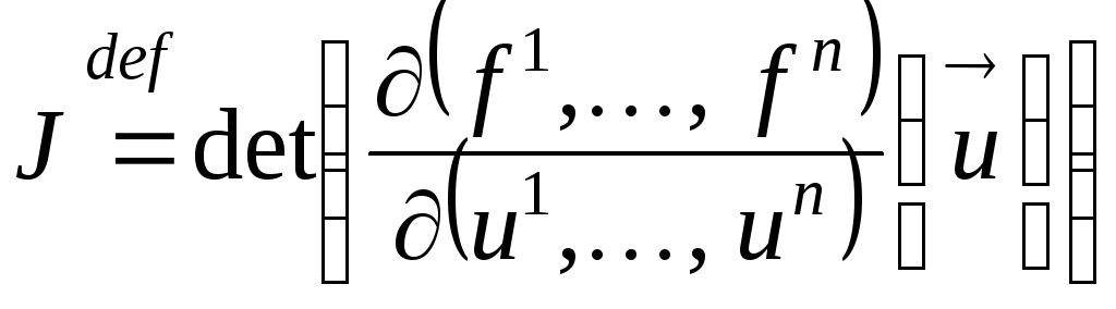
называется
якобианом
преобразования.

Матрицы
Якоби и якобианы называются также
функциональными
матрицами
и функциональными
определителями,
соответственно.

Общее
определение поверхности в евклидовом
пространстве
,
касательная
плоскость.
Рассмотрим два экземпляра пространств

и

с базисами

и

соответственно. Векторы

и

в этих пространствах представляются в
виде разложений

Определение
8.1. Пусть

– некоторая область и

– непрерывно дифференцируемое
отображение. Множество значений

отображения

называется (2-мерной)
элементарной
поверхностью
в пространстве
.

Поверхность
названа элементарной в том смысле, что
она является множеством значений одного
непрерывно дифференцируемого отображения.
Смысл этого замечания состоит в том,
что существуют поверхности, которые не
могут быть определены при помощи одного
отображения.

Из
(8.1) видно, что векторное параметрическое
уравнение поверхности

имеет вид

,
(8.5)

и
эквивалентно скалярным параметрическим
уравнениям

(8.6)

Вектор

называется параметрическим
вектором,
а его координаты – криволинейными
или гауссовскими координатами
на поверхности
,
вектор

называется текущим
или ведущим
вектором поверхности. Дальше будем
предполагать, что компоненты
отображения

дифференцируемы по переменным

нужное число раз.

Если
зафиксирована какая-либо гауссовская
координата в области
,
уравнения (8.5) или (8.6) задают параметризованный
путь, лежащий на поверхности
.
Пусть изменяется
,
а
,
тогда вместо (8.5) или (8.6) имеем

,
(8.7)

(8.7)

Пусть меняется
,
а
,
тогда

,
(8.8)

(8.8)

Так
как компоненты

отображения дифференцируемы по
гауссовским координатам нужное число
раз, пути с уравнениями (8.7) или (8.8)
являются гладкими. Эти пути называются
гауссовскими
координатными линиями на поверхности
.
Если ранг матрицы Якоби

равен 2, то совокупность

системы касательных векторов

(8.9)

путей,
проходящих через точку

и самой точки

поверхности, соответствующей
параметрическому вектору
,
является репером
некоторого двумерного линейного
многообразия.

Определение
8.2. Линейная
оболочка векторов репера

называется касательной
плоскостью
поверхности

в точке
.

Задавая касательные
векторы (8.9) к соответствующим координатным
линиям поверхности в
каждой точке поверхности в виде
,
,
запишем параметрические уравнения
касательной плоскости в виде

После
исключения параметров

и

легко можем получить неявное уравнение
касательной плоскости.

Первая
квадратичная форма поверхности.
Найдём касательный вектор произвольного
пути, проходящего по поверхности

через фиксированную точку
.
Путь зададим при помощи нового параметра
для параметрического вектора
,
положив
,
или
,
,
где
.
Тогда вместо (8.5) имеем:

.
(8.10)

Касательный
вектор находим при помощи правила
дифференцирования сложной функции:

Используя
обозначения (8.9), получаем:

.
(8.11)

Это соотношение
представляет собой разложение
касательного вектора любого пути,
лежащего на поверхности

и проходящего через произвольную точку

поверхности, по направляющим векторам
касательной плоскости – касательным
векторам к гауссовским координатным
линиям,
проходящим через данную точку поверхности.

Длина дуги пути
выражается формулой

.
(8.12)

Из
формулы (8.12) следует, что дифференциал
длины дуги пути может быть вычислен по
формуле:

С
учётом формул (8.9) и (8.11) для произвольного
пути на поверхности получаем:

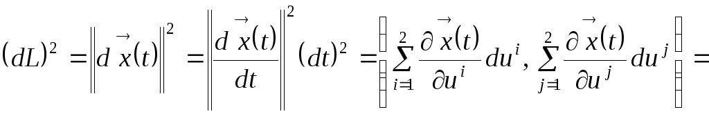
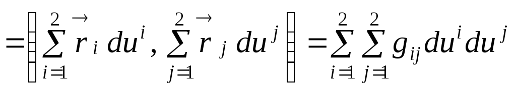Здесь
введены обозначения

(8.13)

для
метрических коэффициентов на поверхности.

Определение
8.3. Пусть

– некоторая поверхность, порождённая
непрерывно дифференцируемым отображением
.
Квадратичная форма

(8.14)

называется
первой
квадратичной формой,
или римановой
метрикой
на поверхности
.

Если известны
функции
,
то подстановка в формулу (8.12) приводит
к следующему результату для длины
пути на поверхности:

.
(8.15)

Для двух пересекающихся
в точке

поверхности

путей с помощью первой квадратичной
формы, если известны функции
,
можно вычислить косинус угла между
касательными векторами путей по формуле

.
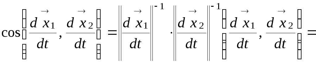
(8.16)

Первая
квадратичная форма (8.14) по построению
является положительно
определённой,
так как определитель её матрицы – это
определитель Грама для линейно независимой
системы векторов.

Для
произвольных векторов

в касательной плоскости имеем следующую
цепочку:

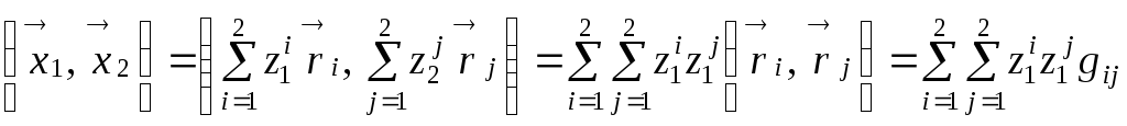Полагая
по определению
,
видим, что скалярное произведение на
поверхности по форме совпадает со
скалярным произведением в обычном
трёхмерном пространстве. Получили
следующий результат.

Источник

«Binormal» redirects here. For the category-theoretic meaning of this word, see normal morphism.

A space curve; the vectors T, N and B; and the osculating plane spanned by T and N

In differential geometry, the Frenet–Serret formulas describe the kinematic properties of a particle moving along a differentiable curve in three-dimensional Euclidean space $mathbb {R} ^{3}$ , or the geometric properties of the curve itself irrespective of any motion. More specifically, the formulas describe the derivatives of the so-called tangent, normal, and binormal unit vectors in terms of each other. The formulas are named after the two French mathematicians who independently discovered them: Jean Frédéric Frenet, in his thesis of 1847, and Joseph Alfred Serret, in 1851. Vector notation and linear algebra currently used to write these formulas were not yet available at the time of their discovery.

The tangent, normal, and binormal unit vectors, often called T, N, and B, or collectively the Frenet–Serret frame or TNB frame, together form an orthonormal basis spanning $mathbb {R} ^{3}$ and are defined as follows:

T is the unit vector tangent to the curve, pointing in the direction of motion.
N is the normal unit vector, the derivative of T with respect to the arclength parameter of the curve, divided by its length.
B is the binormal unit vector, the cross product of T and N.

The Frenet–Serret formulas are:

${displaystyle {begin{aligned}{frac {mathrm {d} mathbf {T} }{mathrm {d} s}}&=kappa mathbf {N} ,\{frac {mathrm {d} mathbf {N} }{mathrm {d} s}}&=-kappa mathbf {T} +tau mathbf {B} ,\{frac {mathrm {d} mathbf {B} }{mathrm {d} s}}&=-tau mathbf {N} ,end{aligned}}}$

where d/ds is the derivative with respect to arclength, κ is the curvature, and τ is the torsion of the curve. The two scalars κ and τ effectively define the curvature and torsion of a space curve. The associated collection, T, N, B, κ, and τ, is called the Frenet–Serret apparatus. Intuitively, curvature measures the failure of a curve to be a straight line, while torsion measures the failure of a curve to be planar.

Definitions[edit]

The T and N vectors at two points on a plane curve, a translated version of the second frame (dotted), and the change in T: δT’. δs is the distance between the points. In the limit $tfrac{dmathbf{T}}{ds}$ will be in the direction N and the curvature describes the speed of rotation of the frame.

Let r(t) be a curve in Euclidean space, representing the position vector of the particle as a function of time. The Frenet–Serret formulas apply to curves which are non-degenerate, which roughly means that they have nonzero curvature. More formally, in this situation the velocity vector r′(t) and the acceleration vector r′′(t) are required not to be proportional.

Let s(t) represent the arc length which the particle has moved along the curve in time t. The quantity s is used to give the curve traced out by the trajectory of the particle a natural parametrization by arc length (i.e. arc-length parametrization), since many different particle paths may trace out the same geometrical curve by traversing it at different rates. In detail, s is given by

${displaystyle s(t)=int _{0}^{t}left|mathbf {r} '(sigma )right|dsigma .}$

Moreover, since we have assumed that r′ ≠ 0, it follows that s(t) is a strictly monotonically increasing function. Therefore, it is possible to solve for t as a function of s, and thus to write r(s) = r(t(s)). The curve is thus parametrized in a preferred manner by its arc length.

With a non-degenerate curve r(s), parameterized by its arc length, it is now possible to define the Frenet–Serret frame (or TNB frame):

The tangent unit vector T is defined as

${displaystyle mathbf {T} :={frac {mathrm {d} mathbf {r} }{mathrm {d} s}}.}$
The normal unit vector N is defined as

${displaystyle mathbf {N} :={{frac {mathrm {d} mathbf {T} }{mathrm {d} s}} over left|{frac {mathrm {d} mathbf {T} }{mathrm {d} s}}right|},}$

from which it follows, since T always has unit magnitude, that N (the change of T) is always perpendicular to T, since there is no change in length of T. Note that by calling curvature ${displaystyle kappa =left|{frac {mathrm {d} mathbf {T} }{mathrm {d} s}}right|}$ we automatically obtain the first relation.

The binormal unit vector B is defined as the cross product of T and N:

The Frenet–Serret frame moving along a helix. The T is represented by the blue arrow, N is represented by the red arrow while B is represented by the black arrow.

from which it follows that B is always perpendicular to both T and N. Thus, the three unit vectors T, N, and B are all perpendicular to each other.

The Frenet–Serret formulas are:

where kappa is the curvature and tau is the torsion.

The Frenet–Serret formulas are also known as Frenet–Serret theorem, and can be stated more concisely using matrix notation:^[1]

${displaystyle {begin{bmatrix}mathbf {T'} \mathbf {N'} \mathbf {B'} end{bmatrix}}={begin{bmatrix}0&kappa &0\-kappa &0&tau \0&-tau &0end{bmatrix}}{begin{bmatrix}mathbf {T} \mathbf {N} \mathbf {B} end{bmatrix}}.}$

This matrix is skew-symmetric.

Formulas in n dimensions[edit]

The Frenet–Serret formulas were generalized to higher-dimensional Euclidean spaces by Camille Jordan in 1874.

Suppose that r(s) is a smooth curve in $mathbb {R} ^{n}$ , and that the first n derivatives of r are linearly independent.^[2] The vectors in the Frenet–Serret frame are an orthonormal basis constructed by applying the Gram-Schmidt process to the vectors (r′(s), r′′(s), …, r⁽ⁿ⁾(s)).

In detail, the unit tangent vector is the first Frenet vector e₁(s) and is defined as

${displaystyle mathbf {e} _{1}(s)={frac {{overline {mathbf {e} _{1}}}(s)}{|{overline {mathbf {e} _{1}}}(s)|}}}$

where

${displaystyle {overline {mathbf {e} _{1}}}(s)=mathbf {r} '(s)}$

The normal vector, sometimes called the curvature vector, indicates the deviance of the curve from being a straight line. It is defined as

$overline{mathbf{e}_2}(s) = mathbf{r}''(s) - langle mathbf{r}''(s), mathbf{e}_1(s) rangle , mathbf{e}_1(s)$

Its normalized form, the unit normal vector, is the second Frenet vector e₂(s) and defined as

$mathbf{e}_2(s) = frac{overline{mathbf{e}_2}(s)} {| overline{mathbf{e}_2}(s) |}$

The tangent and the normal vector at point s define the osculating plane at point r(s).

The remaining vectors in the frame (the binormal, trinormal, etc.) are defined similarly by

${begin{aligned}{mathbf {e}}_{{j}}(s)={frac {overline {{mathbf {e}}_{{j}}}(s)}{|overline {{mathbf {e}}_{{j}}}(s)|}}{mbox{, }}end{aligned}}$

${begin{aligned}overline {{mathbf {e}}_{{j}}}(s)={mathbf {r}}^{{(j)}}(s)-sum _{{i=1}}^{{j-1}}langle {mathbf {r}}^{{(j)}}(s),{mathbf {e}}_{i}(s)rangle ,{mathbf {e}}_{i}(s).end{aligned}}$

The last vector in the frame is defined by the cross-product of the first n-1 vectors:

${displaystyle {mathbf {e} _{n}}(s)={mathbf {e} _{1}}(s)times {mathbf {e} _{2}}(s)times dots times {mathbf {e} _{n-2}}(s)times {mathbf {e} _{n-1}}(s)}$

The real valued functions used below χ_i(s) are called generalized curvature and are defined as

$chi_i(s) = frac{langle mathbf{e}_i'(s), mathbf{e}_{i+1}(s) rangle}{| mathbf{r}'(s) |}$

The Frenet–Serret formulas, stated in matrix language, are

${displaystyle {begin{aligned}{begin{bmatrix}mathbf {e} _{1}'(s)\vdots \mathbf {e} _{n}'(s)\end{bmatrix}}=\end{aligned}}|mathbf {r} '(s)|cdot {begin{aligned}{begin{bmatrix}0&chi _{1}(s)&&0\-chi _{1}(s)&ddots &ddots &\&ddots &0&chi _{n-1}(s)\0&&-chi _{n-1}(s)&0\end{bmatrix}}{begin{bmatrix}mathbf {e} _{1}(s)\vdots \mathbf {e} _{n}(s)\end{bmatrix}}end{aligned}}}$

Notice that as defined here, the generalized curvatures and the frame may differ slightly from the convention found in other sources.
The top curvature ${displaystyle chi _{n-1}}$ (also called the torsion, in this context) and the last vector in the frame ${displaystyle mathbf {e} _{n}}$ ,
differ by a sign

${displaystyle operatorname {or} left(mathbf {r} ^{(1)},dots ,mathbf {r} ^{(n)}right)}$

(the orientation of the basis) from the usual torsion.
The Frenet–Serret formulas are invariant under flipping the sign of both ${displaystyle chi _{n-1}}$ and ${displaystyle mathbf {e} _{n}}$ , and this change of sign makes the frame positively oriented. As defined above, the frame inherits its orientation from the jet of .

Proof[edit]

Consider the 3 by 3 matrix

${displaystyle Q={begin{bmatrix}mathbf {T} \mathbf {N} \mathbf {B} end{bmatrix}}}$

The rows of this matrix are mutually perpendicular unit vectors: an orthonormal basis of $mathbb{R} ^{3}$ . As a result, the transpose of Q is equal to the inverse of Q: Q is an orthogonal matrix. It suffices to show that

${displaystyle left({frac {dQ}{ds}}right)Q^{top }={begin{bmatrix}0&kappa &0\-kappa &0&tau \0&-tau &0end{bmatrix}}}$

Note the first row of this equation already holds, by definition of the normal N and curvature κ, as well as the last row by the definition
of torsion. So it suffices to show that dQ/dsQ^T is a skew-symmetric matrix. Since I = QQ^T, taking a derivative and applying the product rule yields

${displaystyle {begin{aligned}0={frac {mathrm {d} I}{mathrm {d} s}}=left({frac {mathrm {d} Q}{mathrm {d} s}}right)Q^{top }+Qleft({frac {mathrm {d} Q}{mathrm {d} s}}right)^{top }\implies left({frac {mathrm {d} Q}{mathrm {d} s}}right)Q^{top }=-left(left({frac {mathrm {d} Q}{mathrm {d} s}}right)Q^{top }right)^{top }\end{aligned}}}$

which establishes the required skew-symmetry.^[3]

Applications and interpretation[edit]

Kinematics of the frame[edit]

The Frenet–Serret frame moving along a helix in space

The Frenet–Serret frame consisting of the tangent T, normal N, and binormal B collectively forms an orthonormal basis of 3-space. At each point of the curve, this attaches a frame of reference or rectilinear coordinate system (see image).

The Frenet–Serret formulas admit a kinematic interpretation. Imagine that an observer moves along the curve in time, using the attached frame at each point as their coordinate system. The Frenet–Serret formulas mean that this coordinate system is constantly rotating as an observer moves along the curve. Hence, this coordinate system is always non-inertial. The angular momentum of the observer’s coordinate system is proportional to the Darboux vector of the frame.

A top whose axis is situated along the binormal is observed to rotate with angular speed κ. If the axis is along the tangent, it is observed to rotate with angular speed τ.

Concretely, suppose that the observer carries an (inertial) top (or gyroscope) with them along the curve. If the axis of the top points along the tangent to the curve, then it will be observed to rotate about its axis with angular velocity -τ relative to the observer’s non-inertial coordinate system. If, on the other hand, the axis of the top points in the binormal direction, then it is observed to rotate with angular velocity -κ. This is easily visualized in the case when the curvature is a positive constant and the torsion vanishes. The observer is then in uniform circular motion. If the top points in the direction of the binormal, then by conservation of angular momentum it must rotate in the opposite direction of the circular motion. In the limiting case when the curvature vanishes, the observer’s normal precesses about the tangent vector, and similarly the top will rotate in the opposite direction of this precession.

The general case is illustrated below. There are further illustrations on Wikimedia.

Applications[edit]

The kinematics of the frame have many applications in the sciences.

In the life sciences, particularly in models of microbial motion, considerations of the Frenet–Serret frame have been used to explain the mechanism by which a moving organism in a viscous medium changes its direction.^[4]
In physics, the Frenet–Serret frame is useful when it is impossible or inconvenient to assign a natural coordinate system for a trajectory. Such is often the case, for instance, in relativity theory. Within this setting, Frenet–Serret frames have been used to model the precession of a gyroscope in a gravitational well.^[5]

Graphical Illustrations[edit]

Example of a moving Frenet basis (T in blue, N in green, B in purple) along Viviani’s curve.

On the example of a torus knot, the tangent vector T, the normal vector N, and the binormal vector B, along with the curvature κ(s), and the torsion τ(s) are displayed.
At the peaks of the torsion function the rotation of the Frenet–Serret frame (T,N,B) around the tangent vector is clearly visible.

The kinematic significance of the curvature is best illustrated with plane curves (having constant torsion equal to zero). See the page on curvature of plane curves.

Frenet–Serret formulas in calculus[edit]

The Frenet–Serret formulas are frequently introduced in courses on multivariable calculus as a companion to the study of space curves such as the helix. A helix can be characterized by the height 2πh and radius r of a single turn. The curvature and torsion of a helix (with constant radius) are given by the formulas

$kappa = frac{r}{r^2+h^2}$

$tau = pmfrac{h}{r^2+h^2}.$

Two helices (slinkies) in space. (a) A more compact helix with higher curvature and lower torsion. (b) A stretched out helix with slightly higher torsion but lower curvature.

The sign of the torsion is determined by the right-handed or left-handed sense in which the helix twists around its central axis. Explicitly, the parametrization of a single turn of a right-handed helix with height 2πh and radius r is

x = r cos t

y = r sin t

z = h t

(0 ≤ t ≤ 2 π)

and, for a left-handed helix,

x = r cos t

y = −r sin t

z = h t

(0 ≤ t ≤ 2 π).

Note that these are not the arc length parametrizations (in which case, each of x, y, and z would need to be divided by $sqrt{h^2+r^2}$ .)

In his expository writings on the geometry of curves, Rudy Rucker^[6] employs the model of a slinky to explain the meaning of the torsion and curvature. The slinky, he says, is characterized by the property that the quantity

remains constant if the slinky is vertically stretched out along its central axis. (Here 2πh is the height of a single twist of the slinky, and r the radius.) In particular, curvature and torsion are complementary in the sense that the torsion can be increased at the expense of curvature by stretching out the slinky.

Taylor expansion[edit]

Repeatedly differentiating the curve and applying the Frenet–Serret formulas gives the following Taylor approximation to the curve near s = 0:^[7]

${displaystyle mathbf {r} (s)=mathbf {r} (0)+left(s-{frac {s^{3}kappa ^{2}(0)}{6}}right)mathbf {T} (0)+left({frac {s^{2}kappa (0)}{2}}+{frac {s^{3}kappa '(0)}{6}}right)mathbf {N} (0)+left({frac {s^{3}kappa (0)tau (0)}{6}}right)mathbf {B} (0)+o(s^{4}).}$

For a generic curve with nonvanishing torsion, the projection of the curve onto various coordinate planes in the T, N, B coordinate system at s = 0 have the following interpretations:

The osculating plane is the plane containing T and N. The projection of the curve onto this plane has the form:

${displaystyle mathbf {r} (0)+smathbf {T} (0)+{frac {s^{2}kappa (0)}{2}}mathbf {N} (0)+o(s^{2}).}$

This is a parabola up to terms of order o(s²), whose curvature at 0 is equal to κ(0).
The normal plane is the plane containing N and B. The projection of the curve onto this plane has the form:

${displaystyle mathbf {r} (0)+left({frac {s^{2}kappa (0)}{2}}+{frac {s^{3}kappa '(0)}{6}}right)mathbf {N} (0)+left({frac {s^{3}kappa (0)tau (0)}{6}}right)mathbf {B} (0)+o(s^{3})}$

which is a cuspidal cubic to order o(s³).
The rectifying plane is the plane containing T and B. The projection of the curve onto this plane is:

${displaystyle mathbf {r} (0)+left(s-{frac {s^{3}kappa ^{2}(0)}{6}}right)mathbf {T} (0)+left({frac {s^{3}kappa (0)tau (0)}{6}}right)mathbf {B} (0)+o(s^{3})}$

which traces out the graph of a cubic polynomial to order o(s³).

Ribbons and tubes[edit]

A ribbon defined by a curve of constant torsion and a highly oscillating curvature. The arc length parameterization of the curve was defined via integration of the Frenet–Serret equations.

The Frenet–Serret apparatus allows one to define certain optimal ribbons and tubes centered around a curve. These have diverse applications in materials science and elasticity theory,^[8] as well as to computer graphics.^[9]

The Frenet ribbon^[10] along a curve C is the surface traced out by sweeping the line segment [−N,N] generated by the unit normal along the curve. This surface is sometimes confused with the tangent developable, which is the envelope E of the osculating planes of C. This is perhaps because both the Frenet ribbon and E exhibit similar properties along C. Namely, the tangent planes of both sheets of E, near the singular locus C where these sheets intersect, approach the osculating planes of C; the tangent planes of the Frenet ribbon along C are equal to these osculating planes. The Frenet ribbon is in general not developable.

Congruence of curves[edit]

In classical Euclidean geometry, one is interested in studying the properties of figures in the plane which are invariant under congruence, so that if two figures are congruent then they must have the same properties. The Frenet–Serret apparatus presents the curvature and torsion as numerical invariants of a space curve.

Roughly speaking, two curves C and C′ in space are congruent if one can be rigidly moved to the other. A rigid motion consists of a combination of a translation and a rotation. A translation moves one point of C to a point of C′. The rotation then adjusts the orientation of the curve C to line up with that of C′. Such a combination of translation and rotation is called a Euclidean motion. In terms of the parametrization r(t) defining the first curve C, a general Euclidean motion of C is a composite of the following operations:

(Translation) r(t) → r(t) + v, where v is a constant vector.
(Rotation) r(t) + v → M(r(t) + v), where M is the matrix of a rotation.

The Frenet–Serret frame is particularly well-behaved with regard to Euclidean motions. First, since T, N, and B can all be given as successive derivatives of the parametrization of the curve, each of them is insensitive to the addition of a constant vector to r(t). Intuitively, the TNB frame attached to r(t) is the same as the TNB frame attached to the new curve r(t) + v.

This leaves only the rotations to consider. Intuitively, if we apply a rotation M to the curve, then the TNB frame also rotates. More precisely, the matrix Q whose rows are the TNB vectors of the Frenet–Serret frame changes by the matrix of a rotation

A fortiori, the matrix dQ/dsQ^T is unaffected by a rotation:

${displaystyle {frac {mathrm {d} (QM)}{mathrm {d} s}}(QM)^{top }={frac {mathrm {d} Q}{mathrm {d} s}}MM^{top }Q^{top }={frac {mathrm {d} Q}{mathrm {d} s}}Q^{top }}$

since MM^T = I for the matrix of a rotation.

Hence the entries κ and τ of dQ/dsQ^T are invariants of the curve under Euclidean motions: if a Euclidean motion is applied to a curve, then the resulting curve has the same curvature and torsion.

Moreover, using the Frenet–Serret frame, one can also prove the converse: any two curves having the same curvature and torsion functions must be congruent by a Euclidean motion. Roughly speaking, the Frenet–Serret formulas express the Darboux derivative of the TNB frame. If the Darboux derivatives of two frames are equal, then a version of the fundamental theorem of calculus asserts that the curves are congruent. In particular, the curvature and torsion are a complete set of invariants for a curve in three-dimensions.

Other expressions of the frame[edit]

The formulas given above for T, N, and B depend on the curve being given in terms of the arclength parameter. This is a natural assumption in Euclidean geometry, because the arclength is a Euclidean invariant of the curve. In the terminology of physics, the arclength parametrization is a natural choice of gauge. However, it may be awkward to work with in practice. A number of other equivalent expressions are available.

Suppose that the curve is given by r(t), where the parameter t need no longer be arclength. Then the unit tangent vector T may be written as

${displaystyle mathbf {T} (t)={frac {mathbf {r} '(t)}{|mathbf {r} '(t)|}}}$

The normal vector N takes the form

${displaystyle mathbf {N} (t)={frac {mathbf {T} '(t)}{|mathbf {T} '(t)|}}={frac {mathbf {r} '(t)times left(mathbf {r} ''(t)times mathbf {r} '(t)right)}{left|mathbf {r} '(t)right|,left|mathbf {r} ''(t)times mathbf {r} '(t)right|}}}$

The binormal B is then

${displaystyle mathbf {B} (t)=mathbf {T} (t)times mathbf {N} (t)={frac {mathbf {r} '(t)times mathbf {r} ''(t)}{|mathbf {r} '(t)times mathbf {r} ''(t)|}}}$

An alternative way to arrive at the same expressions is to take the first three derivatives of the curve r′(t), r′′(t), r′′′(t), and to apply the Gram-Schmidt process. The resulting ordered orthonormal basis is precisely the TNB frame. This procedure also generalizes to produce Frenet frames in higher dimensions.

In terms of the parameter t, the Frenet–Serret formulas pick up an additional factor of ||r′(t)|| because of the chain rule:

${displaystyle {frac {mathrm {d} }{mathrm {d} t}}{begin{bmatrix}mathbf {T} \mathbf {N} \mathbf {B} end{bmatrix}}=|mathbf {r} '(t)|{begin{bmatrix}0&kappa &0\-kappa &0&tau \0&-tau &0end{bmatrix}}{begin{bmatrix}mathbf {T} \mathbf {N} \mathbf {B} end{bmatrix}}}$

Explicit expressions for the curvature and torsion may be computed. For example,

${displaystyle kappa ={frac {|mathbf {r} '(t)times mathbf {r} ''(t)|}{|mathbf {r} '(t)|^{3}}}}$

The torsion may be expressed using a scalar triple product as follows,

${displaystyle tau ={frac {[mathbf {r} '(t),mathbf {r} ''(t),mathbf {r} '''(t)]}{|mathbf {r} '(t)times mathbf {r} ''(t)|^{2}}}}$

Special cases[edit]

If the curvature is always zero then the curve will be a straight line. Here the vectors N, B and the torsion are not well defined.

If the torsion is always zero then the curve will lie in a plane.

A curve may have nonzero curvature and zero torsion. For example, the circle of radius R given by r(t)=(R cos t, R sin t, 0) in the z=0 plane has zero torsion and curvature equal to 1/R. The converse, however, is false. That is, a regular curve with nonzero torsion must have nonzero curvature. (This is just the contrapositive of the fact that zero curvature implies zero torsion.)

A helix has constant curvature and constant torsion.

Plane curves[edit]

Given a curve contained on the x—y plane, its tangent vector T is also contained on that plane. Its binormal vector B can be naturally postulated to coincide with the normal to the plane (along the z axis). Finally, the curve normal can be found completing the right-handed system, N = B × T.^[11] This form is well-defined even when the curvature is zero; for example, the normal to a straight line in a plane will be perpendicular to the tangent, all co-planar.

Notes[edit]

^ Kühnel 2002, §1.9
^ Only the first n − 1 actually need to be linearly independent, as the final remaining frame vector e_n can be chosen as the unit vector orthogonal to the span of the others, such that the resulting frame is positively oriented.
^ This proof is likely due to Élie Cartan. See Griffiths (1974) where he gives the same proof, but using the Maurer-Cartan form. Our explicit description of the Maurer-Cartan form using matrices is standard. See, for instance, Spivak, Volume II, p. 37. A generalization of this proof to n dimensions is not difficult, but was omitted for the sake of exposition. Again, see Griffiths (1974) for details.
^ Crenshaw (1993).
^ Iyer and Vishveshwara (1993).
^ Rucker, Rudy (1999). «Watching Flies Fly: Kappatau Space Curves». San Jose State University. Archived from the original on 15 October 2004.
^ Kühnel 2002, p. 19
^ Goriely et al. (2006).
^ Hanson.
^ For terminology, see Sternberg (1964). Lectures on Differential Geometry. Englewood Cliffs, N.J., Prentice-Hall. p. 252-254. ISBN 9780135271506..
^ Weisstein, Eric W. «Normal Vector». MathWorld. Wolfram.

References[edit]

Crenshaw, H.C.; Edelstein-Keshet, L. (1993), «Orientation by Helical Motion II. Changing the direction of the axis of motion», Bulletin of Mathematical Biology, 55 (1): 213–230, doi:10.1016/s0092-8240(05)80070-9, S2CID 50734771
Etgen, Garret; Hille, Einar; Salas, Saturnino (1995), Salas and Hille’s Calculus — One and Several Variables (7th ed.), John Wiley & Sons, p. 896
Frenet, F. (1847), Sur les courbes à double courbure (PDF), Thèse, Toulouse. Abstract in Journal de Mathématiques Pures et Appliquées 17, 1852.
Goriely, A.; Robertson-Tessi, M.; Tabor, M.; Vandiver, R. (2006), «Elastic growth models», BIOMAT-2006 (PDF), Springer-Verlag, archived from the original (PDF) on 2006-12-29.
Griffiths, Phillip (1974), «On Cartan’s method of Lie groups and moving frames as applied to uniqueness and existence questions in differential geometry», Duke Mathematical Journal, 41 (4): 775–814, doi:10.1215/S0012-7094-74-04180-5, S2CID 12966544.
Guggenheimer, Heinrich (1977), Differential Geometry, Dover, ISBN 0-486-63433-7
Hanson, A.J. (2007), «Quaternion Frenet Frames: Making Optimal Tubes and Ribbons from Curves» (PDF), Indiana University Technical Report
Iyer, B.R.; Vishveshwara, C.V. (1993), «Frenet-Serret description of gyroscopic precession», Phys. Rev., D, 48 (12): 5706–5720, arXiv:gr-qc/9310019, Bibcode:1993PhRvD..48.5706I, doi:10.1103/physrevd.48.5706, PMID 10016237, S2CID 119458843
Jordan, Camille (1874), «Sur la théorie des courbes dans l’espace à n dimensions», C. R. Acad. Sci. Paris, 79: 795–797
Kühnel, Wolfgang (2002), Differential geometry, Student Mathematical Library, vol. 16, Providence, R.I.: American Mathematical Society, ISBN 978-0-8218-2656-0, MR 1882174
Serret, J. A. (1851), «Sur quelques formules relatives à la théorie des courbes à double courbure» (PDF), Journal de Mathématiques Pures et Appliquées, 16.
Spivak, Michael (1999), A Comprehensive Introduction to Differential Geometry (Volume Two), Publish or Perish, Inc..
Sternberg, Shlomo (1964), Lectures on Differential Geometry, Prentice-Hall
Struik, Dirk J. (1961), Lectures on Classical Differential Geometry, Reading, Mass: Addison-Wesley.

External links[edit]

Create your own animated illustrations of moving Frenet-Serret frames, curvature and torsion functions (Maple Worksheet)
Rudy Rucker’s KappaTau Paper.
Very nice visual representation for the trihedron

Источник

Содержание

Касательная, нормальная плоскость, соприкасающаяся плоскость, бинормаль, главная нормаль, репер Френе

Краткие теоретические сведения

Кривая в пространстве

Касательная к кривой

Нормальная плоскость

Соприкасающаяся плоскость

Бинормаль и главная нормаль

Спрямляющая плоскость

Репер Френе

Решение задач

Задача 1

Решение задачи 1

Задача 2

Решение задачи 2

Задача 3

Решение задачи 3

Definitions[edit]

Formulas in n dimensions[edit]

Proof[edit]

Applications and interpretation[edit]

Kinematics of the frame[edit]

Applications[edit]

Graphical Illustrations[edit]

Frenet–Serret formulas in calculus[edit]

Taylor expansion[edit]

Ribbons and tubes[edit]

Congruence of curves[edit]

Other expressions of the frame[edit]

Special cases[edit]

Plane curves[edit]

See also[edit]

Notes[edit]

References[edit]

External links[edit]

Не пропустите также: