Укажите размеры:
Результат:
Решение:
![]()
Ссылка на страницу с результатом:
# Теория
Прямоугольный треугольник — это геометрическая фигура, образованная тремя отрезками соединяющихся тремя точками, у которой все углы внутренние, при этом один из углов прямой (равен 90°).
β
α
a
b
c
Тангенс угла tg(α) — это тригонометрическая функция выражающая отношение противолежащего катета a к прилежащему катету b.
Формула тангенса
tg alpha = dfrac{a}{b}
- tg α — тангенс угла α
- a — противолежащий катет
- b — прилежащий катет
Арктангенс — это обратная тригонометрическая функция. Арктангенсом числа x называется такое значение угла α, выраженное в радианах, для которого tg α = x. Вычислить арктангенс, означает найти угол α, тангенс которого равен числу x.
Углы треугольника
Сумма углов треугольника всегда равна 180 градусов:
angle alpha + angle beta + angle gamma = 180°
Так как у прямоугольного треугольника один из углов равен 90°, то сумма двух других углов равна 90°.
Поэтому, если известен один из острых углов треугольника, второй угол можно посчитать по формуле:
angle alpha = 90° — angle beta
angle beta = 90° — angle alpha
Острый угол — угол, значение которого меньше 90°.
У прямоугольного треугольника один угол прямой, а два других угла — острые.
Похожие калькуляторы:
Войдите чтобы писать комментарии
- Определение
-
График арктангенса
- Свойства арктангенса
- Таблица арктангенсов
Определение
Арктангенс (arctg или arctan) – это обратная тригонометрическая функция.
Арктангенс x определяется как функция, обратная к тангенсу x, где x – любое число (x∈ℝ).
Если тангенс угла у равен х (tg y = x), значит арктангенс x равняется y:
arctg x = tg-1 x = y, причем -π/2<y<π/2
Примечание: tg-1x означает обратный тангенс, а не тангенс в степени -1.
Например:
arctg 1 = tg-1 1 = 45° = π/4 рад
График арктангенса
Функция арктангенса пишется как y = arctg (x). График в общем виде выглядит следующим образом:

Свойства арктангенса
Ниже в табличном виде представлены основные свойства арктангенса с формулами.
Таблица арктангенсов
| arctg x (°) | arctg x (рад) | x |
| -90° | -π/2 | -∞ |
| -71.565° | -1.2490 | -3 |
| -63.435° | -1.1071 | -2 |
| -60° | -π/3 | -√3 |
| -45° | -π/4 | -1 |
| -30° | -π/6 | -1/√3 |
| -26.565° | -0.4636 | -0.5 |
| 0° | 0 | 0 |
| 26.565° | 0.4636 | 0.5 |
| 30° | π/6 | 1/√3 |
| 45° | π/4 | 1 |
| 60° | π/3 | √3 |
| 63.435° | 1.1071 | 2 |
| 71.565° | 1.2490 | 3 |
| 90° | π/2 | ∞ |
microexcel.ru
При решении геодезических и инженерных задач, очень часто приходиться вспоминать и искать необходимые формулы. В связи с этим хочется представить Вам шпаргалку (назовем её “геодезической шпаргалкой”:)), в которой приведены часто использующиеся формулы.
Конечно, ее содержание не охватывает всю высшую математику или сферическую геометрию, но что-нибудь должно пригодиться.
Зная из собственного опыта, неудобство восприятия формул без чисел, к каждой из них приводится пример вычисления.
Теорема Пифагора

Пример вычислений теорема Пифагора

Соотношения в прямоугольном треугольнике

Пример вычислений соотношения в прямоугольном треугольнике

Обратные тригонометрические функции арксинус (arcsin), арккосинус (arccos), арктангенс (arctg) и арккотангенс (arcctg)
— арксинус (arcsin) возвращает угол по его синусу
— арккосинус (arccos) возвращает угол по его косинусу
— арктангенс (arctg) возвращает угол по его тангенсу
— арккотангенс (arcctg) возвращает угол по его арктангенсу
Пример вычислений обратные тригонометрические функции

Сумма углов треугольника
Сумма углов в треугольнике равна 180 градусам

Теорема синусов
Для любого треугольника соблюдается выражение

Пример вычислений теорема синусов

Теорема косинусов
Квадрат любой стороны треугольника, равен сумме квадратов двух других его сторон, минус удвоенное произведение этих сторон на косинус угла между ними

Пример вычислений теорема косинусов

Площадь треугольника
Площадь треугольника можно определить по формулам

также удобно использовать формулу Герона  ,
,
где p-полупериметр треугольника 
Пример вычислений площадь треугольника

или по формуле Герона

Площадь круга

Длина дуги окружности
Длина дуги окружности вычисляется по формулам
 если угол задан в угловых градусах минутах и секундах
 если угол задан в радианах
Пример вычислений длина дуги окружности
угол задан в угловых градусах минутах и секундах

угол задан в радианах

Перевод градусов в угловые градусы минуты и секунды
Перевод угловых градусов минут и секунд в градусы выполняется согласно выражения

Пример вычислений
перевести в градусы угол, который задан в угловых градусах минутах и секундах


Перевод градусов в угловые градусы минуты и секунды
Перевод градусов в угловые градусы минуты и секунды выполняется согласно выражения
Пример вычислений
перевести в угловые градусы минуты и секунды угол, который задан в градусах


Перевод градусов в радианы
Перевод градусов в радианы выполняется по формуле

Пример вычислений
перевести в радианы угол, который задан в угловых градусах минутах и секундах


Перевод радианов в градусы
Перевод радианов в градусы выполняется по формуле

Пример вычислений
перевести в угловые градусы минуты и секунды угол, который задан в радианах


Определение наклона линии в градусах
Определение наклона линии в градусах выполняется с использованием соотношений в прямоугольном треугольнике
Пример вычислений
Определить наклон пандуса длиной 14м и высотой 3,5м

Определение уклона линии в долях, процентах и промилле
При инженерно-строительных работах, наклон линии задают не градусом наклона, а тангенсом этого градуса — безразмерной величиной, которая называется уклоном. Уклон может выражаться относительным числом, в процентах (сотые доли числа) и промилле (тысячные доли числа)
Пример вычислений
Определить уклон отмостки длиной 2,5м и высотой 0,30м

In mathematics, the inverse trigonometric functions (occasionally also called arcus functions,[1][2][3][4][5] antitrigonometric functions[6] or cyclometric functions[7][8][9]) are the inverse functions of the trigonometric functions (with suitably restricted domains). Specifically, they are the inverses of the sine, cosine, tangent, cotangent, secant, and cosecant functions,[10] and are used to obtain an angle from any of the angle’s trigonometric ratios. Inverse trigonometric functions are widely used in engineering, navigation, physics, and geometry.
Notation[edit]
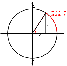
For a circle of radius 1, arcsin and arccos are the lengths of actual arcs determined by the quantities in question.
Several notations for the inverse trigonometric functions exist. The most common convention is to name inverse trigonometric functions using an arc- prefix: arcsin(x), arccos(x), arctan(x), etc.[6] (This convention is used throughout this article.) This notation arises from the following geometric relationships:[citation needed]
when measuring in radians, an angle of θ radians will correspond to an arc whose length is rθ, where r is the radius of the circle. Thus in the unit circle, «the arc whose cosine is x» is the same as «the angle whose cosine is x«, because the length of the arc of the circle in radii is the same as the measurement of the angle in radians.[11] In computer programming languages, the inverse trigonometric functions are often called by the abbreviated forms asin, acos, atan.[12]
The notations sin−1(x), cos−1(x), tan−1(x), etc., as introduced by John Herschel in 1813,[13][14] are often used as well in English-language sources,[6] much more than the also established sin[−1](x), cos[−1](x), tan[−1](x) – conventions consistent with the notation of an inverse function, that is useful (for example) to define the multivalued version of each inverse trigonometric function:  However, this might appear to conflict logically with the common semantics for expressions such as sin2(x) (although only sin2 x, without parentheses, is the really common use), which refer to numeric power rather than function composition, and therefore may result in confusion between notation for the reciprocal (multiplicative inverse) and inverse function.[15]
The confusion is somewhat mitigated by the fact that each of the reciprocal trigonometric functions has its own name — for example, (cos(x))−1 = sec(x). Nevertheless, certain authors advise against using it, since it is ambiguous.[6][16] Another precarious convention used by a small number of authors is to use an uppercase first letter, along with a “−1” superscript: Sin−1(x), Cos−1(x), Tan−1(x), etc.[17] Although it is intended to avoid confusion with the reciprocal, which should be represented by sin−1(x), cos−1(x), etc., or, better, by sin−1 x, cos−1 x, etc., it in turn creates yet another major source of ambiguity, especially since many popular high-level programming languages (e.g. Mathematica, and MAGMA) use those very same capitalised representations for the standard trig functions, whereas others (Python, SymPy, NumPy, Matlab, MAPLE, etc.) use lower-case.
Hence, since 2009, the ISO 80000-2 standard has specified solely the «arc» prefix for the inverse functions.
Basic concepts[edit]
Principal values[edit]
Since none of the six trigonometric functions are one-to-one, they must be restricted in order to have inverse functions. Therefore, the result ranges of the inverse functions are proper (i.e. strict) subsets of the domains of the original functions.
For example, using function in the sense of multivalued functions, just as the square root function  could be defined from
  the function
  is defined so that
  For a given real number
  with
with  there are multiple (in fact, countably infinitely many) numbers
  such that
  ; for example,
  but also
 etc. When only one value is desired, the function may be restricted to its principal branch. With this restriction, for each
  in the domain, the expression
  will evaluate only to a single value, called its principal value. These properties apply to all the inverse trigonometric functions.
The principal inverses are listed in the following table.
| Name | Usual notation | Definition | Domain of for real result
|
Range of usual principal value (radians) |
Range of usual principal value (degrees) |
|---|---|---|---|---|---|
| arcsine | |
x = sin(y) |  |
 |

|
| arccosine |  |
x = cos(y) | |
 |

|
| arctangent |  |
x = tan(y) | all real numbers |  |

|
| arccotangent |  |
x = cot(y) | all real numbers |  |

|
| arcsecant |  |
x = sec(y) |  |
 |

|
| arccosecant |  |
x = csc(y) | |
 |

|
Note: Some authors[citation needed] define the range of arcsecant to be  , because the tangent function is nonnegative on this domain. This makes some computations more consistent. For example, using this range,
  whereas with the range
  , we would have to write
  since tangent is nonnegative on
  but nonpositive on
  For a similar reason, the same authors define the range of arccosecant to be
  or
or 
If is allowed to be a complex number, then the range of applies only to its real part.
The table below displays names and domains of the inverse trigonometric functions along with the range of their usual principal values in radians.
| Name | Symbol | Domain | Image/Range | Inverse function |
Domain | Image of principal values |
||||
|---|---|---|---|---|---|---|---|---|---|---|
| sine | 
|

|

|

|
![[-1, 1]](https://wikimedia.org/api/rest_v1/media/math/render/svg/51e3b7f14a6f70e614728c583409a0b9a8b9de01)
|

|
|
|
|
![{displaystyle left[-{tfrac {pi }{2}},{tfrac {pi }{2}}right]}](https://wikimedia.org/api/rest_v1/media/math/render/svg/c2052f9d4a9c6a14f6db2e4bcd2606bce26d720d)
|
| cosine | 
|
|
|
|
|

|
|
|
|
![[0,pi ]](https://wikimedia.org/api/rest_v1/media/math/render/svg/3e2a912eda6ef1afe46a81b518fe9da64a832751)
|
| tangent | 
|
|

|
|
|

|
|
|
|

|
| cotangent | 
|
|

|
|
|

|
|
|
|

|
| secant | 
|
|
|
|

|

|
|
|
|
![{displaystyle [,0,;pi ,];;;setminus left{{tfrac {pi }{2}}right}}](https://wikimedia.org/api/rest_v1/media/math/render/svg/c913c2c78d11f57ccd118976bfb4b0595e5a2e0e)
|
| cosecant | 
|
|
|
|
|

|
|
|
|
![{displaystyle left[-{tfrac {pi }{2}},{tfrac {pi }{2}}right]setminus {0}}](https://wikimedia.org/api/rest_v1/media/math/render/svg/e84fda7925743a03ffa0aec3fbed76a2967a3012)
|
The symbol  denotes the set of all real numbers and
  denotes the set of all integers. The set of all integer multiples of
  is denoted by

The symbol  denotes set subtraction so that, for instance,
 ![{displaystyle mathbb {R} setminus (-1,1)=(-infty ,-1]cup [1,infty )}](https://wikimedia.org/api/rest_v1/media/math/render/svg/105fc2887189c9dbf0d165542a768dcd97f03069) is the set of points in (that is, real numbers) that are not in the interval
is the set of points in (that is, real numbers) that are not in the interval 
The Minkowski sum notation  and
and  that is used above to concisely write the domains of
  is now explained.
Domain of cotangent and cosecant :
The domains of  and
and  are the same. They are the set of all angles
  at which
  i.e. all real numbers that are not of the form
  for some integer

Domain of tangent and secant :
The domains of  and
and  are the same. They are the set of all angles at which

Solutions to elementary trigonometric equations[edit]
Each of the trigonometric functions is periodic in the real part of its argument, running through all its values twice in each interval of  :
:
This periodicity is reflected in the general inverses, where  is some integer.
The following table shows how inverse trigonometric functions may be used to solve equalities involving the six standard trigonometric functions.
It is assumed that the given values 

 and all lie within appropriate ranges so that the relevant expressions below are well-defined.
Note that «for some  » is just another way of saying «for some integer
  »
»
The symbol  is logical equality. The expression «LHS RHS» indicates that either (a) the left hand side (i.e. LHS) and right hand side (i.e. RHS) are both true, or else (b) the left hand side and right hand side are both false; there is no option (c) (e.g. it is not possible for the LHS statement to be true and also simultaneously for the RHS statement to false), because otherwise «LHS RHS» would not have been written (see this footnote[note 1] for an example illustrating this concept).
| Equation | if and only if | Solution | Expanded form of solution | where… | |||||||
|---|---|---|---|---|---|---|---|---|---|---|---|

|

|

|

|

|

|

|
for some
|
|
 or or 
|
for some 
|
|

|
|
|
|

|
|
|
for some
|
|
 or or 
|
for some
|
|

|
|
|

|

|
|

|
|
for some
|
|
 or or 
|
for some
|

|
|
|
|

|
|
|
|
for some
|
|
 or or 
|
for some
|

|
|
|

|
|
|
for some
|
|||||

|
|
|

|
|
|
for some
|
For example, if  then
then  for some
  While if
  then
then  for some
  where will be even if
  and it will be odd if
  The equations
  and
and  have the same solutions as and
  respectively. In all equations above except for those just solved (i.e. except for / and /), the integer in the solution’s formula is uniquely determined by (for fixed
  and ).
- Detailed example and explanation of the «plus or minus» symbol

The solutions to and  involve the «plus or minus» symbol
  whose meaning is now clarified. Only the solution to will be discussed since the discussion for is the same.
We are given between and we know that there is an angle in some interval that satisfies  We want to find this
  The table above indicates that the solution is

which is a shorthand way of saying that (at least) one of the following statement is true:
- for some integer
or - for some integer


As mentioned above, if  (which by definition only happens when
  ) then both statements (1) and (2) hold, although with different values for the integer : if
  is the integer from statement (1), meaning that
  holds, then the integer for statement (2) is
  (because
  ).
).
However, if  then the integer is unique and completely determined by
If  (which by definition only happens when
  ) then
  (because
  and
and  so in both cases
  is equal to
  ) and so the statements (1) and (2) happen to be identical in this particular case (and so both hold).
Having considered the cases and  we now focus on the case where
  and
and  So assume this from now on. The solution to is still
which as before is shorthand for saying that one of statements (1) and (2) is true. However this time, because and  statements (1) and (2) are different and furthermore, exactly one of the two equalities holds (not both). Additional information about is needed to determine which one holds. For example, suppose that
  and that all that is known about is that
  (and nothing more is known). Then

and moreover, in this particular case  (for both the
  case and the
  case) and so consequently,

This means that could be either  or
or  Without additional information it is not possible to determine which of these values has.
An example of some additional information that could determine the value of would be knowing that the angle is above the -axis (in which case  ) or alternatively, knowing that it is below the -axis (in which case
  ).
).
Transforming equations
The equations above can be transformed by using the reflection and shift identities:[18]
Argument: 
|

|

|

|

|

|
 , where , where
|
|||||
|---|---|---|---|---|---|---|---|---|---|---|---|

|
|

|

|

|

|
|
|
|

|
|
|

|
|
|

|

|
|
|
|
|
|
|
|

|
|
|
|
|
|
|
|
|
|
||

|
|
|
|
|
|
|
|
|
|
||

|
|
|

|
|

|
|
|
|
|
|
|

|
|
|
|
|
|
|
|
|
|
|
|
These formulas imply, in particular, that the following hold:
![{displaystyle {begin{alignedat}{28}sin theta &=-&&sin(-theta )&&=-&&sin(pi +theta )&&=&&sin(pi -theta )&&=-&&cos {Big (}{frac {pi }{2}}+theta {Big )}&&=;&&cos {Big (}{frac {pi }{2}}-theta {Big )}&&=-&&cos {Big (}-{frac {pi }{2}}-theta {Big )}&&=&&cos {Big (}-{frac {pi }{2}}+theta {Big )}&&=-&&cos {bigg (}{frac {3pi }{2}}-theta {bigg )}&&=-&&cos {bigg (}-{frac {3pi }{2}}+theta {bigg )}\[0.3ex]cos theta &=&&cos(-theta )&&=-&&cos(pi +theta )&&=&&cos(pi -theta )&&=&&sin {Big (}{frac {pi }{2}}+theta {Big )}&&=&&sin {Big (}{frac {pi }{2}}-theta {Big )}&&=-&&sin {Big (}-{frac {pi }{2}}-theta {Big )}&&=-&&sin {Big (}-{frac {pi }{2}}+theta {Big )}&&=-&&sin {bigg (}{frac {3pi }{2}}-theta {bigg )}&&=&&sin {bigg (}-{frac {3pi }{2}}+theta {bigg )}\[0.3ex]tan theta &=-&&tan(-theta )&&=&&tan(pi +theta )&&=-&&tan(pi -theta )&&=-&&cot {Big (}{frac {pi }{2}}+theta {Big )}&&=&&cot {Big (}{frac {pi }{2}}-theta {Big )}&&=&&cot {Big (}-{frac {pi }{2}}-theta {Big )}&&=-&&cot {Big (}-{frac {pi }{2}}+theta {Big )}&&=&&cot {bigg (}{frac {3pi }{2}}-theta {bigg )}&&=-&&cot {bigg (}-{frac {3pi }{2}}+theta {bigg )}\[0.3ex]end{alignedat}}}](https://wikimedia.org/api/rest_v1/media/math/render/svg/cef665382b8d7a245e102a633458de97a2ba8aa0)
where swapping  swapping
  and swapping
  gives the analogous equations for
  respectively.
So for example, by using the equality  the equation can be transformed into
  which allows for the solution to the equation
  (where
  ) to be used; that solution being:

which becomes:

where using the fact that  and substituting
  proves that another solution to
  is:
is:

The substitution  may be used express the right hand side of the above formula in terms of
  instead of
Equal identical trigonometric functions[edit]
The table below shows how two angles and  must be related if their values under a given trigonometric function are equal or negatives of each other.
| Equation | if and only if | Solution | where… | Also a solution to | ||||||||
|---|---|---|---|---|---|---|---|---|---|---|---|---|
|
|
|

|
|

|
|
|
|
|
for some
|

|
||
|
|
|

|
|
|
|
|
|
|
|
for some
|

|
|
|
|
|

|
|
|
|
|
|
for some
|

|
|||

|
|
|
|
|

|
|
|
|
for some
|

|
||

|
|
|
|
|
|
|
|
|
|

|
for some
|

|

|
|
|
|
|
|
|
|
|
for some
|

|
||

|
|

|
|
|
|
|
|
|
for some
|

|
||
| ⇕ | ||||||||||||

|
|

|
Relationships between trigonometric functions and inverse trigonometric functions[edit]
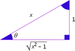
Trigonometric functions of inverse trigonometric functions are tabulated below. A quick way to derive them is by considering the geometry of a right-angled triangle, with one side of length 1 and another side of length then applying the Pythagorean theorem and definitions of the trigonometric ratios. Purely algebraic derivations are longer.[citation needed] It is worth noting that for arcsecant and arccosecant, the diagram assumes that is positive, and thus the result has to be corrected through the use of absolute values and the signum (sgn) operation.
|
|

|

|

|
Diagram |
|---|---|---|---|---|
|
|

|

|

|

|
|
|

|

|

|

|

|

|

|

|

|

|

|

|

|

|

|

|

|

|

|

|

|

|

|
|
Relationships among the inverse trigonometric functions[edit]
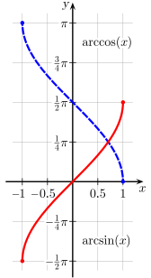
The usual principal values of the arcsin(x) (red) and arccos(x) (blue) functions graphed on the cartesian plane.

The usual principal values of the arctan(x) and arccot(x) functions graphed on the cartesian plane.

Principal values of the arcsec(x) and arccsc(x) functions graphed on the cartesian plane.
Complementary angles:
![{begin{aligned}arccos(x)&={frac {pi }{2}}-arcsin(x)\[0.5em]operatorname {arccot}(x)&={frac {pi }{2}}-arctan(x)\[0.5em]operatorname {arccsc}(x)&={frac {pi }{2}}-operatorname {arcsec}(x)end{aligned}}](https://wikimedia.org/api/rest_v1/media/math/render/svg/ec43798232f580abb074cf15f3d77692edd36af0)
Negative arguments:

Reciprocal arguments:
![{displaystyle {begin{aligned}arccos left({frac {1}{x}}right)&=operatorname {arcsec}(x)\[0.3em]arcsin left({frac {1}{x}}right)&=operatorname {arccsc}(x)\[0.3em]arctan left({frac {1}{x}}right)&={frac {pi }{2}}-arctan(x)=operatorname {arccot}(x),,{text{ if }}x>0\[0.3em]arctan left({frac {1}{x}}right)&=-{frac {pi }{2}}-arctan(x)=operatorname {arccot}(x)-pi ,,{text{ if }}x<0\[0.3em]operatorname {arccot} left({frac {1}{x}}right)&={frac {pi }{2}}-operatorname {arccot}(x)=arctan(x),,{text{ if }}x>0\[0.3em]operatorname {arccot} left({frac {1}{x}}right)&={frac {3pi }{2}}-operatorname {arccot}(x)=pi +arctan(x),,{text{ if }}x<0\[0.3em]operatorname {arcsec} left({frac {1}{x}}right)&=arccos(x)\[0.3em]operatorname {arccsc} left({frac {1}{x}}right)&=arcsin(x)end{aligned}}}](https://wikimedia.org/api/rest_v1/media/math/render/svg/ecb0a376d9148e3cf65ea6e6ed5fb37752a581c7)
Useful identities if one only has a fragment of a sine table:

Whenever the square root of a complex number is used here, we choose the root with the positive real part (or positive imaginary part if the square was negative real).
A useful form that follows directly from the table above is
- .

It is obtained by recognizing that  .
.
From the half-angle formula,  , we get:
![{displaystyle {begin{aligned}arcsin(x)&=2arctan left({frac {x}{1+{sqrt {1-x^{2}}}}}right)\[0.5em]arccos(x)&=2arctan left({frac {sqrt {1-x^{2}}}{1+x}}right),,{text{ if }}-1<xleq 1\[0.5em]arctan(x)&=2arctan left({frac {x}{1+{sqrt {1+x^{2}}}}}right)end{aligned}}}](https://wikimedia.org/api/rest_v1/media/math/render/svg/7dd6a9370a877ca5e198e28b7582bd06b377bdc3)
Arctangent addition formula[edit]

This is derived from the tangent addition formula

by letting

In calculus[edit]
Derivatives of inverse trigonometric functions[edit]
The derivatives for complex values of z are as follows:

Only for real values of x:

For a sample derivation: if  , we get:

Expression as definite integrals[edit]
Integrating the derivative and fixing the value at one point gives an expression for the inverse trigonometric function as a definite integral:

When x equals 1, the integrals with limited domains are improper integrals, but still well-defined.
Infinite series[edit]
Similar to the sine and cosine functions, the inverse trigonometric functions can also be calculated using power series, as follows. For arcsine, the series can be derived by expanding its derivative,  , as a binomial series, and integrating term by term (using the integral definition as above). The series for arctangent can similarly be derived by expanding its derivative
  in a geometric series, and applying the integral definition above (see Leibniz series).
![{displaystyle {begin{aligned}arcsin(z)&=z+left({frac {1}{2}}right){frac {z^{3}}{3}}+left({frac {1cdot 3}{2cdot 4}}right){frac {z^{5}}{5}}+left({frac {1cdot 3cdot 5}{2cdot 4cdot 6}}right){frac {z^{7}}{7}}+cdots \[5pt]&=sum _{n=0}^{infty }{frac {(2n-1)!!}{(2n)!!}}{frac {z^{2n+1}}{2n+1}}\[5pt]&=sum _{n=0}^{infty }{frac {(2n)!}{(2^{n}n!)^{2}}}{frac {z^{2n+1}}{2n+1}},;qquad |z|leq 1end{aligned}}}](https://wikimedia.org/api/rest_v1/media/math/render/svg/a0f778db7f760db059cf12f13ee5c2bf239fbb2f)

Series for the other inverse trigonometric functions can be given in terms of these according to the relationships given above. For example,  ,
,  , and so on. Another series is given by:[19]

Leonhard Euler found a series for the arctangent that converges more quickly than its Taylor series:
- [20]

(The term in the sum for n = 0 is the empty product, so is 1.)
Alternatively, this can be expressed as

Another series for the arctangent function is given by

where  is the imaginary unit.[21]
Continued fractions for arctangent[edit]
Two alternatives to the power series for arctangent are these generalized continued fractions:

The second of these is valid in the cut complex plane. There are two cuts, from −i to the point at infinity, going down the imaginary axis, and from i to the point at infinity, going up the same axis. It works best for real numbers running from −1 to 1. The partial denominators are the odd natural numbers, and the partial numerators (after the first) are just (nz)2, with each perfect square appearing once. The first was developed by Leonhard Euler; the second by Carl Friedrich Gauss utilizing the Gaussian hypergeometric series.
Indefinite integrals of inverse trigonometric functions[edit]
For real and complex values of z:
![{displaystyle {begin{aligned}int arcsin(z),dz&{}=z,arcsin(z)+{sqrt {1-z^{2}}}+C\int arccos(z),dz&{}=z,arccos(z)-{sqrt {1-z^{2}}}+C\int arctan(z),dz&{}=z,arctan(z)-{frac {1}{2}}ln left(1+z^{2}right)+C\int operatorname {arccot}(z),dz&{}=z,operatorname {arccot}(z)+{frac {1}{2}}ln left(1+z^{2}right)+C\int operatorname {arcsec}(z),dz&{}=z,operatorname {arcsec}(z)-ln left[zleft(1+{sqrt {frac {z^{2}-1}{z^{2}}}}right)right]+C\int operatorname {arccsc}(z),dz&{}=z,operatorname {arccsc}(z)+ln left[zleft(1+{sqrt {frac {z^{2}-1}{z^{2}}}}right)right]+Cend{aligned}}}](https://wikimedia.org/api/rest_v1/media/math/render/svg/e3e2dde92bb82231c4326e45ce8b50e7298688bb)
For real x ≥ 1:

For all real x not between -1 and 1:

The absolute value is necessary to compensate for both negative and positive values of the arcsecant and arccosecant functions. The signum function is also necessary due to the absolute values in the derivatives of the two functions, which create two different solutions for positive and negative values of x. These can be further simplified using the logarithmic definitions of the inverse hyperbolic functions:

The absolute value in the argument of the arcosh function creates a negative half of its graph, making it identical to the signum logarithmic function shown above.
All of these antiderivatives can be derived using integration by parts and the simple derivative forms shown above.
Example[edit]
Using  (i.e. integration by parts), set

Then

which by the simple substitution  yields the final result:

Extension to complex plane[edit]

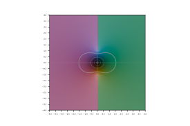
A Riemann surface for the argument of the relation tan z = x. The orange sheet in the middle is the principal sheet representing arctan x. The blue sheet above and green sheet below are displaced by 2π and −2π respectively.
Since the inverse trigonometric functions are analytic functions, they can be extended from the real line to the complex plane. This results in functions with multiple sheets and branch points. One possible way of defining the extension is:

where the part of the imaginary axis which does not lie strictly between the branch points (−i and +i) is the branch cut between the principal sheet and other sheets. The path of the integral must not cross a branch cut. For z not on a branch cut, a straight line path from 0 to z is such a path. For z on a branch cut, the path must approach from Re[x] > 0 for the upper branch cut and from Re[x] < 0 for the lower branch cut.
The arcsine function may then be defined as:

where (the square-root function has its cut along the negative real axis and) the part of the real axis which does not lie strictly between −1 and +1 is the branch cut between the principal sheet of arcsin and other sheets;

which has the same cut as arcsin;

which has the same cut as arctan;

where the part of the real axis between −1 and +1 inclusive is the cut between the principal sheet of arcsec and other sheets;

which has the same cut as arcsec.
Logarithmic forms[edit]
These functions may also be expressed using complex logarithms. This extends their domains to the complex plane in a natural fashion. The following identities for principal values of the functions hold everywhere that they are defined, even on their branch cuts.
![{displaystyle {begin{aligned}arcsin(z)&{}=-iln left({sqrt {1-z^{2}}}+izright)=iln left({sqrt {1-z^{2}}}-izright)&{}=operatorname {arccsc} left({frac {1}{z}}right)\[10pt]arccos(z)&{}=-iln left(i{sqrt {1-z^{2}}}+zright)={frac {pi }{2}}-arcsin(z)&{}=operatorname {arcsec} left({frac {1}{z}}right)\[10pt]arctan(z)&{}=-{frac {i}{2}}ln left({frac {i-z}{i+z}}right)=-{frac {i}{2}}ln left({frac {1+iz}{1-iz}}right)&{}=operatorname {arccot} left({frac {1}{z}}right)\[10pt]operatorname {arccot}(z)&{}=-{frac {i}{2}}ln left({frac {z+i}{z-i}}right)=-{frac {i}{2}}ln left({frac {iz-1}{iz+1}}right)&{}=arctan left({frac {1}{z}}right)\[10pt]operatorname {arcsec}(z)&{}=-iln left(i{sqrt {1-{frac {1}{z^{2}}}}}+{frac {1}{z}}right)={frac {pi }{2}}-operatorname {arccsc}(z)&{}=arccos left({frac {1}{z}}right)\[10pt]operatorname {arccsc}(z)&{}=-iln left({sqrt {1-{frac {1}{z^{2}}}}}+{frac {i}{z}}right)=iln left({sqrt {1-{frac {1}{z^{2}}}}}-{frac {i}{z}}right)&{}=arcsin left({frac {1}{z}}right)end{aligned}}}](https://wikimedia.org/api/rest_v1/media/math/render/svg/13b511be341b52fcd0c0660f3a4b1e5a164bfcb1)
Generalization[edit]
Because all of the inverse trigonometric functions output an angle of a right triangle, they can be generalized by using Euler’s formula to form a right triangle in the complex plane. Algebraically, this gives us:

or

where  is the adjacent side,
  is the opposite side, and
  is the hypotenuse. From here, we can solve for .

or

Simply taking the imaginary part works for any real-valued and , but if or is complex-valued, we have to use the final equation so that the real part of the result isn’t excluded. Since the length of the hypotenuse doesn’t change the angle, ignoring the real part of  also removes from the equation. In the final equation, we see that the angle of the triangle in the complex plane can be found by inputting the lengths of each side. By setting one of the three sides equal to 1 and one of the remaining sides equal to our input
  , we obtain a formula for one of the inverse trig functions, for a total of six equations. Because the inverse trig functions require only one input, we must put the final side of the triangle in terms of the other two using the Pythagorean Theorem relation

The table below shows the values of a, b, and c for each of the inverse trig functions and the equivalent expressions for that result from plugging the values into the equations above and simplifying.

In order to match the principal branch of the natural log and square root functions to the usual principal branch of the inverse trig functions, the particular form of the simplified formulation matters. The formulations given in the two rightmost columns assume ![{displaystyle operatorname {Im} left(ln zright)in (-pi ,pi ]}](https://wikimedia.org/api/rest_v1/media/math/render/svg/781cef7f2317c18794eeaaddeef4073aadd51b75) and
and  . To match the principal branch
  and
and  to the usual principal branch of the inverse trig functions, subtract from the result when
  .
.
In this sense, all of the inverse trig functions can be thought of as specific cases of the complex-valued log function. Since these definition work for any complex-valued , the definitions allow for hyperbolic angles as outputs and can be used to further define the inverse hyperbolic functions. Elementary proofs of the relations may also proceed via expansion to exponential forms of the trigonometric functions.
Example proof[edit]

Using the exponential definition of sine, and letting 
![{displaystyle {begin{aligned}z&={frac {e^{iphi }-e^{-iphi }}{2i}}\[10mu]2iz&=xi -{frac {1}{xi }}\[5mu]0&=xi ^{2}-2izxi -1\[5mu]xi &=izpm {sqrt {1-z^{2}}}\[5mu]phi &=-iln left(izpm {sqrt {1-z^{2}}}right)end{aligned}}}](https://wikimedia.org/api/rest_v1/media/math/render/svg/ed03e8cf773fa44cc78823d65f7d82f41276fb96)
(the positive branch is chosen)


|

|
|

|

|

|

|

|

|

|

|

|
Applications[edit]
Finding the angle of a right triangle[edit]

Inverse trigonometric functions are useful when trying to determine the remaining two angles of a right triangle when the lengths of the sides of the triangle are known. Recalling the right-triangle definitions of sine and cosine, it follows that

Often, the hypotenuse is unknown and would need to be calculated before using arcsine or arccosine using the Pythagorean Theorem:  where
where  is the length of the hypotenuse. Arctangent comes in handy in this situation, as the length of the hypotenuse is not needed.

For example, suppose a roof drops 8 feet as it runs out 20 feet. The roof makes an angle θ with the horizontal, where θ may be computed as follows:

In computer science and engineering[edit]
Two-argument variant of arctangent[edit]
The two-argument atan2 function computes the arctangent of y / x given y and x, but with a range of (−π, π]. In other words, atan2(y, x) is the angle between the positive x-axis of a plane and the point (x, y) on it, with positive sign for counter-clockwise angles (upper half-plane, y > 0), and negative sign for clockwise angles (lower half-plane, y < 0). It was first introduced in many computer programming languages, but it is now also common in other fields of science and engineering.
In terms of the standard arctan function, that is with range of (−π/2, π/2), it can be expressed as follows:

It also equals the principal value of the argument of the complex number x + iy.
This limited version of the function above may also be defined using the tangent half-angle formulae as follows:

provided that either x > 0 or y ≠ 0. However this fails if given x ≤ 0 and y = 0 so the expression is unsuitable for computational use.
The above argument order (y, x) seems to be the most common, and in particular is used in ISO standards such as the C programming language, but a few authors may use the opposite convention (x, y) so some caution is warranted. These variations are detailed at atan2.
Arctangent function with location parameter[edit]
In many applications[22] the solution of the equation  is to come as close as possible to a given value
  . The adequate solution is produced by the parameter modified arctangent function

The function  rounds to the nearest integer.
Numerical accuracy[edit]
For angles near 0 and π, arccosine is ill-conditioned, and similarly with arcsine for angles near −π/2 and π/2. Computer applications thus need to consider the stability of inputs to these functions and the sensitivity of their calculations, or use alternate methods.[23]
See also[edit]
- Arcsine distribution
- Inverse exsecant
- Inverse versine
- Inverse hyperbolic functions
- List of integrals of inverse trigonometric functions
- List of trigonometric identities
- Trigonometric function
- Trigonometric functions of matrices
Notes[edit]
- ^ To clarify, suppose that it is written «LHS RHS» where LHS (which abbreviates left hand side) and RHS are both statements that can individually be either be true or false. For example, if and are some given and fixed numbers and if the following is written:
then LHS is the statement «
«. Depending on what specific values and have, this LHS statement can either be true or false. For instance, LHS is true if and (because in this case ) but LHS is false if and (because in this case which is not equal to ); more generally, LHS is false if and Similarly, RHS is the statement « for some «. The RHS statement can also either true or false (as before, whether the RHS statement is true or false depends on what specific values and have). The logical equality symbol means that (a) if the LHS statement is true then the RHS statement is also necessarily true, and moreover (b) if the LHS statement is false then the RHS statement is also necessarily false. Similarly, also means that (c) if the RHS statement is true then the LHS statement is also necessarily true, and moreover (d) if the RHS statement is false then the LHS statement is also necessarily false.


References[edit]
- Abramowitz, Milton; Stegun, Irene A., eds. (1972). Handbook of Mathematical Functions with Formulas, Graphs, and Mathematical Tables. New York: Dover Publications. ISBN 978-0-486-61272-0.
- ^ Taczanowski, Stefan (1 October 1978). «On the optimization of some geometric parameters in 14 MeV neutron activation analysis». Nuclear Instruments and Methods. ScienceDirect. 155 (3): 543–546. Bibcode:1978NucIM.155..543T. doi:10.1016/0029-554X(78)90541-4.
- ^ Hazewinkel, Michiel (1994) [1987]. Encyclopaedia of Mathematics (unabridged reprint ed.). Kluwer Academic Publishers / Springer Science & Business Media. ISBN 978-155608010-4.
- ^ Ebner, Dieter (25 July 2005). Preparatory Course in Mathematics (PDF) (6 ed.). Department of Physics, University of Konstanz. Archived (PDF) from the original on 26 July 2017. Retrieved 26 July 2017.
- ^ Mejlbro, Leif (11 November 2010). Stability, Riemann Surfaces, Conformal Mappings — Complex Functions Theory (PDF) (1 ed.). Ventus Publishing ApS / Bookboon. ISBN 978-87-7681-702-2. Archived from the original (PDF) on 26 July 2017. Retrieved 26 July 2017.
- ^ Durán, Mario (2012). Mathematical methods for wave propagation in science and engineering. Vol. 1: Fundamentals (1 ed.). Ediciones UC. p. 88. ISBN 978-956141314-6.
- ^ a b c d Hall, Arthur Graham; Frink, Fred Goodrich (January 1909). «Chapter II. The Acute Angle [14] Inverse trigonometric functions». Written at Ann Arbor, Michigan, USA. Trigonometry. Vol. Part I: Plane Trigonometry. New York, USA: Henry Holt and Company / Norwood Press / J. S. Cushing Co. — Berwick & Smith Co., Norwood, Massachusetts, USA. p. 15. Retrieved 12 August 2017.
[…] α = arcsin m: It is frequently read «arc-sine m» or «anti-sine m,» since two mutually inverse functions are said each to be the anti-function of the other. […] A similar symbolic relation holds for the other trigonometric functions. […] This notation is universally used in Europe and is fast gaining ground in this country. A less desirable symbol, α = sin-1m, is still found in English and American texts. The notation α = inv sin m is perhaps better still on account of its general applicability. […]
- ^ Klein, Christian Felix (1924) [1902]. Elementarmathematik vom höheren Standpunkt aus: Arithmetik, Algebra, Analysis (in German). Vol. 1 (3rd ed.). Berlin: J. Springer.
- ^ Klein, Christian Felix (2004) [1932]. Elementary Mathematics from an Advanced Standpoint: Arithmetic, Algebra, Analysis. Translated by Hedrick, E. R.; Noble, C. A. (Translation of 3rd German ed.). Dover Publications, Inc. / The Macmillan Company. ISBN 978-0-48643480-3. Retrieved 13 August 2017.
- ^ Dörrie, Heinrich (1965). Triumph der Mathematik. Translated by Antin, David. Dover Publications. p. 69. ISBN 978-0-486-61348-2.
- ^ Weisstein, Eric W. «Inverse Trigonometric Functions». mathworld.wolfram.com. Retrieved 29 August 2020.
- ^ Beach, Frederick Converse; Rines, George Edwin, eds. (1912). «Inverse trigonometric functions». The Americana: a universal reference library. Vol. 21.
- ^ Cook, John D. (11 February 2021). «Trig functions across programming languages». johndcook.com (blog). Retrieved 10 March 2021.
- ^ Cajori, Florian (1919). A History of Mathematics (2 ed.). New York, NY: The Macmillan Company. p. 272.
- ^ Herschel, John Frederick William (1813). «On a remarkable Application of Cotes’s Theorem». Philosophical Transactions. Royal Society, London. 103 (1): 8. doi:10.1098/rstl.1813.0005.
- ^ «Inverse trigonometric functions». Wiki. Brilliant Math & Science (brilliant.org). Retrieved 29 August 2020.
- ^ Korn, Grandino Arthur; Korn, Theresa M. (2000) [1961]. «21.2.-4. Inverse Trigonometric Functions». Mathematical handbook for scientists and engineers: Definitions, theorems, and formulars for reference and review (3 ed.). Mineola, New York, USA: Dover Publications, Inc. p. 811. ISBN 978-0-486-41147-7.
- ^ Bhatti, Sanaullah; Nawab-ud-Din; Ahmed, Bashir; Yousuf, S. M.; Taheem, Allah Bukhsh (1999). «Differentiation of Trigonometric, Logarithmic and Exponential Functions». In Ellahi, Mohammad Maqbool; Dar, Karamat Hussain; Hussain, Faheem (eds.). Calculus and Analytic Geometry (1 ed.). Lahore: Punjab Textbook Board. p. 140.
- ^ Abramowitz & Stegun 1972, p. 73, 4.3.44
- ^ Borwein, Jonathan; Bailey, David; Gingersohn, Roland (2004). Experimentation in Mathematics: Computational Paths to Discovery (1 ed.). Wellesley, MA, USA: A. K. Peters. p. 51. ISBN 978-1-56881-136-9.
- ^ Hwang Chien-Lih (2005), «An elementary derivation of Euler’s series for the arctangent function», The Mathematical Gazette, 89 (516): 469–470, doi:10.1017/S0025557200178404, S2CID 123395287
- ^ S. M. Abrarov and B. M. Quine (2018), «A formula for pi involving nested radicals», The Ramanujan Journal, 46 (3): 657–665, arXiv:1610.07713, doi:10.1007/s11139-018-9996-8, S2CID 119150623
- ^ when a time varying angle crossing should be mapped by a smooth line instead of a saw toothed one (robotics, astromomy, angular movement in general)[citation needed]
- ^ Gade, Kenneth (2010). «A non-singular horizontal position representation» (PDF). The Journal of Navigation. Cambridge University Press. 63 (3): 395–417. Bibcode:2010JNav…63..395G. doi:10.1017/S0373463309990415.

External links[edit]
- Weisstein, Eric W. «Inverse Tangent». MathWorld.